The following theorem supplies the basic elements necessary for construction of generalized fractal interpolation functions.

Theorem 1. Let the interpolating data set D = {P_i = [x_i  y_i  z_i]^T Î R³, x_i < x_i+1, i = 0, 1,.., n}(n ³ 2)  be given. Consider the IFS s(D) = {R ³; w₁,..., w_n}, where  w_i are given by (1) with

and the real numbers  d_i, h_i, l_i, m_i  are parameters chosen such that w_i (i = 1,..., n ) are contractive mappings.  Then, the limiting set

is the graph of a continuous vector valued function  f : [x₀, x_n] ® R² having the interpolation property  f(x_i) = [ y_i  z_i]^T ,  i = 0,1,..., n.

Proof.  It is straightforward to see that, with the special choice of  e_i, f_i, g_i  given here, the transformations in the IFS take the form
 

which give immediately   w_i(P₀) = P_i-1,  and  w_i(P_n) = P_i   for any  i = 1,2,..., n. The rest of the proof  follows from Theorems 4.1 and 4.2  in [3, ch. VI ].  à

For  i = 1,..,n, denote by M_i the sub-matrix of  A_i  whose elements are d_i, h_i, l_i, m_i
 

                                               (6)

The conditions that  d_i, h_i, l_i, m_i  must obey in order that a transformation of the form of  w_i  Îs(D) be a contraction, are given in the following lemma.

Lemma 1.   A transformation w_i  having  the form (1)with  a_i < 1   is a contraction of  R³ if and only if the elements  d_i, h_i, l_i, m_i  of  A_i satisfy one of the following two systems of inequalities
 

Proof.  Denote the spectral radius of a matrix  M  by r(M). Then
 

is a necessary and sufficient condition for the mapping w_i to be a contraction w.r.t. a feasible metric d in R ³.

Let  Q_i = (d_i-m_i)² + 4 h_i l_i , and let l₁(i) , l₂(i) , l₃(i)  denote the eigenvalues of  the matrix  A_i  in (2),  more precisely  let l₁ (i) = a_i, l₂(i)= ¹/₂( d_i+ m_i -  ÖQ_i ) and l₃(i)= ¹/₂( d_i+ m_i+  ÖQ_i). Then, (8) is equivalent to

Let Q_i  ³ 0 ( this is equivalent to the first inequality in the first system in the assertion ). Then, l₂(i) , l₃(i) Î R,  and  l₂(i) £ l₃(i).So the condition {|l₂(i)| < 1 Ù |l₃(i)| < 1 } is equivalent to { -1 < l₂(i)  Ù  l₃(i) < 1 }, or  {ÖQ_i  < d_i + m_i + 2   Ù   ÖQ_i < -d_i-m_i + 2} which, in turn, is equivalent to the set of inequalities

By squaring both sides of  both  left inequalities and  replacing  Q_i = (d_i-m_i)² + 4 h_i l_i, the  above set  reduces to the second  inequality of (7a).

If, instead,  Q_i  < 0, the first inequality in the second system is satisfied. Furthermore, in this case  l₂(i) and l₃(i) are conjugate complex numbers having common modulus  |l₂(i)|  =  |l₃(i)| =  ¹/₂| d_i + m_i + i Ö(-Q_i )|  = ¹/₂ Ö[(d_i+m_i)²- Q_i ], therefore  the condition {|l₂(i)| < 1  Ù |l₃(i)| < 1} yields  Ö[ (d_i+m_i)²- Q_i ] < 2  which reduces to Ö(d_im_i-h_i l_i) < 1,  and to the second  inequality of (7b), which is thereby completely proved. à

The folowing corollary gives the condition on matrices  M_i ( i = 1,..,n) under which the IFS is hyperbolic.

Corollary 1. The IFS s(D) = {R³; w₁, ..., w_n}, built according to the rules given in Theorem 1,  is hyperbolic if and only if for all  i = 1,..., n  the elements of the parameter matrix M_i satisfy the conditions (7a) and (7b).

Proof. It is straightforward since the hypotheses made in Theorem 1 about  D yield a_i < 1 ( i = 1,.. ,n) and, therefore, Lemma 1 applies. à

Let us denote  by M the set of all the parameter matrices in the IFS  s(D), M = {M_i, i = 1,..,n}. It is clear, now,  that the uniqueness of the attractor of s(D) and, of course, the shape of the attractor itself depend on the parameter matrices M just as well as on the interpolation data D. Therefore, in the following, whenever this dependence will be relevant to our discussion we will introduce the set of parameter matrices in our notation, denoting by  s(D,M) the corresponding IFS.  Also we will denote by the same symbol  the corresponding  interpolation scheme, namely the rule by  which the continuous vector valued function  f , being the unique attractor of  s(D,M), is associated  to D.

Example 1. Consider the data set D= {(0, 0, 0), (1/4, 0, 1/2), (1/2, 1/2, 1), (3/4, 1, 1/2), (1, 1, 0)}. By Theorem 1, a four term IFS s(D) = {R ³; w₁, w₂, w₃, w₄}, such that its attractor is the graph of a vector valued fractal interpolation  function f, can be associated to D. If  the items of {M_i , i = 1,..,4} are chosen, for example, to be :  d₁ = d₂= 1/2, d₃ = -1/4, d₄ = 0; h₁ = h₄ = 1/4, h₂ = -1/4, h₃ = 1/2; l₁ = l₄ = 1/4,  l₂ = l₃ = -1/4; m₁ = 0, m₂ = 1/4,  m₃ = -1/4, m₄ =1/2, then the affine mappings w₁, w₂, w₃, w₄   have the form  (2), with

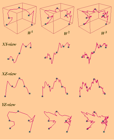
Direct checking shows that this choice of  d_i, h_i, l_i, m_i  satisfies constraints in  Lemma 1, so the coefficient matrices above define contractive linear mappings R ³® R ³. Indeed, one could also evaluate directly r( A₁) = r( A₄) = (1+ Ö2 )/4 » 0.603553,   r(A₂) = ( 3 + Ö5 )/8 » 0.654508,  and r(A₃) = Ö3 /4 » 0.433013,  to discover that all are smaller than 1, which guarantees that the IFS s(D) is hyperbolic and its attractor F_D is unique.

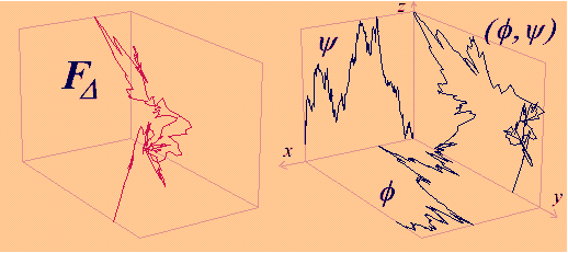
In Figure 1 (top) the preattractors W ¹(G), W ²(G) and W ³(G) are displayed, where G is the piecewise linear interpolant of D. The rest of Fig. 1 shows the projections of these preattractors on the coordinate planes. The interpolating points are marked in all projections.

Figure 2 (left)  shows the attractor of the orbit of  G, this is F_D =  {[x f(x) y(x)]^T, x ÎI= [0,1]} which is the graph of   f (x) = [f(x) y(x)]^T . The projections of  F_D on the coordinate planes,  f ={ [x f(x)]^T, xÎI}, y={[x y(x)]^T, xÎI}and the parametric curve  f = (f,y) are shown in Figure 2 (right). The functions f and y are called hidden variable fractal interpolation functions (Barnsley [2], [3], Massopust [14]) meaning that they depend on the "third variable" that is not present in the plane containing their graphs.

In fact they do share the interpolation property of F_Dbut, while F_D is, by its own nature, a self affine set, in the general case the projections f and y are not self affine.