Decorative Knotting Using Trigonometric Parametrizations.

By Lindsay D Taylor

Introduction

This document describes the formation of decorative and interesting knots using computer 3-D graphics. It is written from the perspective of the practicalities of pattern design, not mathematical theory. The approach uses trigonometric parameterizations for the knots and is based on the use of epitrochoid and hypotrochoid plane curves interlaced by using one or more sin functions in the 3^rd dimension. In its simplest form they can be represented by the following equations.

                    |

                     |         Equations 1

                                                     |

for

p, q are non-zero integers and  When  the loops face outwards, while when the loops face inwards.

The form used for the x and y equations was derived from that used by Edwards (1) who produced a staggering and oftentimes bewildering range of complex and intricate decorative patterns for 2-D computer graphics in emulation of those produced in the 18^th and 19^th centuries using the “Geometric Lathe” and the Spirograph® toy (2) of the 1960’s.

Figure 1 shows an interlaced compound triple knot formed by the procedures described in this document.

Figure 1 - Compound Triple Knot

Methodology

The patterns were realized using Blender 3D (3). Blender 3D is a free 3D graphics application which has been released under the terms of the GNU General Public License. It is available for multiple operating systems and contains a feature set comparable with high-end commercial 3D graphics software. One of the strengths of Blender is that it comes with an embedded Python interpreter, which allows it to run scripts written in that programming language. These scripts can use the Blender/Python application programming interface (API) to expand Blender's functionality

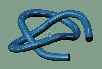
Figure 2 - Surface creation from NURBS curve

The patterns were generated as NURBS curves generated by a Python script. A NURBS curve is defined in terms of a set of “control points” which define a “control polygon”. The curves were then turned into virtual 3D objects using an “extrude along path” technique.  This consists of creating a surface by sweeping a separately-created profile along the curved path by assigning a Bevel Object (BevOb) to the curve. A visualization of the process can be seen in Figure 2.

Results and Discussion

Torus Knots using Outward-Looping Curves

The Trefoil Knot

A wide range of torus knots can be prepared using the above-described simple equations. That is to say, without the use of the standard equations used to describe a torus knot (4).

The Trefoil Knot, when considered as a simple outward facing loop pattern (), requires separate handling and will be considered first. It can be described by the following equations:

Figure 3 shows a Trefoil Knot ( and demonstrates the effect of varying the ratio in Equations 1. When  (in this case 0.5) a cusped pattern results. Above this value a looped pattern is produced with the inner curves touching when . Above this value the loops intersect producing the familiar Trefoil Knot pattern.

It should be noted that the Torus Knot (and the circulating patterns which follow) can also be represented by the more familiar form of the x, y equations representing a hypocycloid curve. That is to say,  and the sign change in the x equation as shown below also results in a Trefoil Knot.:

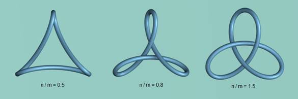
Figure 3 - Trefoil Knot

Torus Knots using “Outer Circulating Patterns”.

For the following patterns the value of p is increased. In the days of the “Mechanical Lathe” the x-y plane patterns of this type were known as circulating patterns because they took more than one cycle to get back to the starting point. When considered in terms of 3-D knot patterns this is the most basic definition of a torus knot. If , the equations generate standard torus knots. The requirement for p and q to be relatively prime still stands.

It is interesting that the first pattern formed in this fashion also generate a Trefoil Knot as seen by the following equations:

With this type of pattern the number of loops is equal to  and the number of cycles taken to return to the starting point is p. Figure 4 and Figure 5 show groups of torus knots. The equations used for their production follow:

(2, 7) Knot

            xval = cos(2*θ) + 0.2*cos(-5* θ)

yval = sin(2* θ) + 0.2*sin(-5* θ)

            zval = 0.35*sin(7* θ)

(2,9) Knot

xval = cos(2* θ) + 0.25*cos(-7* θ)

            yval = sin(2* θ) + 0.25*sin(-7* θ)

zval = 0.35*sin(9* θ)

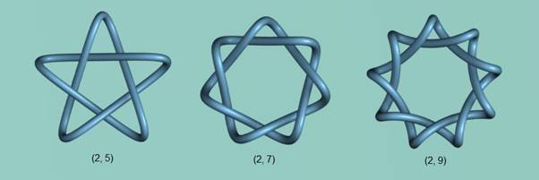
Figure 4 - Some Torus Knots

The procedure can produce knots with  as can be seen with the series of knots shown in Figure 5.

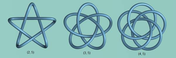
Figure 5 - Five Loop Series of Torus Knots

(2, 5) Knot

(3, 5) Knot

(4, 5) Knot

The data presented here show a procedure for generating torus knots without the use of the standard equations. In this respect, Kauffman (5) has previously shown that all Torus Knots can be expressed as Fourier Knots of the form Fourier-(1, 3, 3) and Hoste (6) that their simplest representation is as Fourier-(1,1,2) knots. Thus, it is not surprising that many Torus Knots, when derived from a different viewpoint, can also be represented as Fourier-(1, 2, 2) knots as is shown in this document. The equations shown above have the limitation that they are not universal for all Torus Knots (viz Figure Eight Knot) and are not as intuitive to use as the standard equations for Torus Knots.

The Figure Eight Knot and other Inner Looping Patterns

The following patterns share the feature that

Figure Eight Knot

Figure 6 shows three knots which apparently share a similar underlying structure. The first is the Figure Eight Knot. Since, in this case, the inner loops are required to intersect . The knot can be described by the following simple set of equations.

Figure 6a

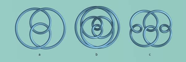
Figure 6 - Figure Eight and Similar Knots

Figure 6b is an inner circulating pattern (p = 2) while Figure 6c, although simpler in appearance than Figure 6b is, in fact, an example of a compound knot. More examples of this type of knot will be given in the next section. 

Figure 6b

Figure 6c

Inner Circulating Patterns

Inner circulating patterns have the characteristic of having . Figure 7 shows three such patterns with n/m < 1. Inspection shows that Figure 7a and Figure 7b have the appearance of decorated torus knots which return to their starting point in two cycles. That this type of equation does represent a torus knot is easily demonstrated by reducing the n/m ratio as is shown in Figure 8 where  was reduced to 0.3 in the equations for Figure 7a (and  used in the z equation). It is clear from this and other work (5), (7) that there are several conceptual ways to define a Trefoil Knot (and other Torus Knots).

Figure 7c shows an example where q = 3. It is an interesting pattern as it has three inner and outer loops and also takes three cycles to return to the starting position.

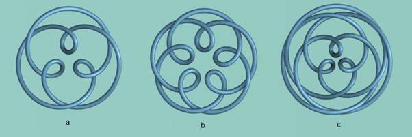
Figure 7 - Inner Circulating Patterns

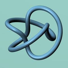
Figure 8 - Trefoil Knot using "Inner Loops"

Figure 7a

Figure 7b

Figure 7c

Some Compound Patterns

Compound patterns are those in which an additional trig function has been added to the x and y equations. Only a single aspect of this broad area will be examined here – patterns made from groups of simple knots.

Pairs of Knots.

The simplest examples of this are the Granny Knot and Square Knot which are both pairs of 3-crossing knots. Inspection of Figure 9 demonstrates that these two knots share the same x,y pattern and merely differ in their interlacing. Thus, they can be formed using the same x,y equations and merely altering the z equation. These equations are distinct and simpler than those described by Trautwein (7) who used a more organic and complex 3-dimensional approach to knot design which used both cos and sin functions in all three equations.

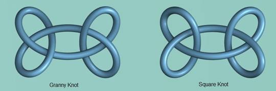
Figure 9 - The Square and Granny Knots

For the Granny Knot the following z equation is used:

while for the Square Knot the corresponding equation is:

An alternative, simpler, set of equations for the Granny Knot follows. It is based on a four outer loop pattern with intersecting central curve

Knot pairs need not be limited to 3-crossing knots. Figure 10 shows two related examples of pairs of 4-crossing knots. Figure 10b is probably the simplest form for equations describing a pair of 4-crossing knots.

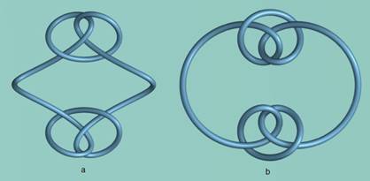
Figure 10 - 4-Crossing Knot Pairs

Figure 10a

)

Figure 10b

Larger Groupings of Knots

An advantage of the more 2-dimensional approach to knot design used in this document is that it can be used to produce larger grouping of knots using relatively minor alterations to the equations. Some results of this can be seen in Figure 1 and Figure 11 and Figure 12

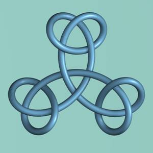
Figure 11 - A Compound Triple Knot

Figure 11 Equations

The following style of knot (Figure 12) has been created with from between three and six outer knots by minor alterations to the equations.

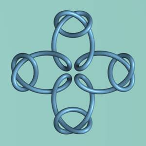
Figure 12 - A Compound Quadruple Knot

Figure 12 Equations

A Note on the Interlacing of Patterns

The approach to interlacing patterns used in this document was simple – the use of a sine function. Although it can be used to successfully produce fully-interlaced patterns in a variety of patterns, it is a naïve approach. The simplest approach, which is to use a number of sine waves in the z equation which equal the number of crossings, can fail in even a very simple knot. This occurs most frequently when there are regions in the pattern where the crossings are near each other while they are distant in other regions of the pattern. In some cases better interlacing can be obtained by the addition of an additional sin function in the z equation to modulate its shape. This approach was used in the production of several of the knots described in this document. Alternatively, increasing the frequency of the sine waves can often produce a successfully interlaced pattern but results in an ugly pattern. This problem is illustrated in Figure 13.

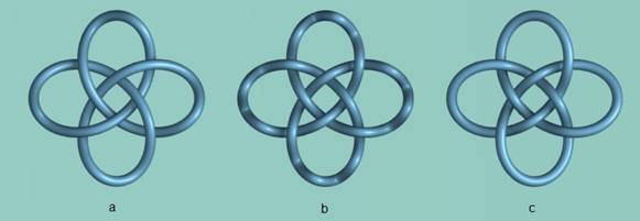
Figure 13 - Interlacing problems and a solution

The simple four outer loop pattern is shown with three interlacing solutions. In Figure 13a. the interlacing fails when  – the number of crossings. In Figure 13b when  was used, a successfully interlaced pattern was achieved but also resulted in the presence of unnecessary waves in the outer regions of the pattern.

This difficulty can be seen in many of the patterns produced by Morita (8) , which used this method of curve interlacing. It should be noted that in his work the additional curves were, in some cases, used to advantage when the individual pattern was used as a unit of a larger pattern!

A pragmatic solution to many of these problems can be achieved by a minor recoding of the script which generates the pattern to have a different frequency of the sine wave in different regions of the pattern - see Figure 13c. The following extract of the script code demonstrates this solution by the use of an if…else conditional statement when calculating the z equation.

xval = cos(pi*u) + 1.5*cos(-3*pi*u)

            yval = sin(pi*u) + 1.5*sin(-3*pi*u)

            if 0.167 < u < 0.333 or 0.666 < u < 0.834 or \

            1.167 < u < 1.333 or 1.667 < u < 1.834:

                        zval = 0.35*sin(16*pi*u)

            else:

                        zval = 0.35*sin(4*pi*u)

A more elegant solution to the problem can be achieved in many cases by creating patterns which use fully-interlaced torus knots. This procedure is described in the accompanying document.

Works Cited

1. Edwards, Ross. Microcomputer Art. Australia : Prentice-Hall, 1985. ISBN 0 7248 0795 0.

2. Weisstein, Eric W. Spirograph. From MathWorld--A Wolfram Web Resource. http://mathworld.wolfram.com/Spirograph.html.

3. Blender 3D. http://www.blender.org/ . [Online] The Blender Foundation.

4. Torus Knot. From Wikipedia, the free encyclopedia. http://en.wikipedia.org/wiki/Torus_knot.

5. Kauffman, Louis H. Fourier Knots. http://www.math.uic.edu/~kauffman/PJFourier.pdf.

6. Hoste, Jim. Torus Knots are Fourier-(1, 1, 2) Knots. 2008. arXiv:0708.3590v1.

7. Trautwein, Aaron. Harmonic Knots. Ph. D Thesis. July 1995. Department of Mathematics, University of Iowa, Iowa City, Iowa, U.S.A.

8. Morita, Katsumi. Shapes of Knot Patterns. Forma. 2007, Vol. 22, pp. 75-91.