Integration by Parts: a Visual Proof

Sasho Kalajdzievski
Department of Mathematics
University of Manitoba
sacho@cc.UManitoba.CA

1. Introduction.

    If is a Riemann integrable function with respect to over the interval [a,b] then is Riemann integrable with respect to over [a,b], and we have the so called Integration by Parts Formula (in the setting of Riemann-Stieltjes integrals):

.      (*)

    We assume below that and have continuous derivatives in [a,b]. Under that assumption, Riemann-Stieltjes integral reduces to Riemann integral, and (*) can be interpreted as the more elementary (Riemann) Integration by Parts Formula, where stands for (and stands for ).We provide a visual justification of the formula (for both Riemann and Riemann-Stieltjes integrals).

2. Proof.

    In the pictures we present, both and are increasing and positive. The other combinations of monotonic functions can be handled similarly, with due care for the sign of the terms corresponding to areas of the rectangular regions we use below. Without going into details, we notice that the general case can be reduced to the preceding by subdividing the interval [a,b] into subintervals over each of which and are monotonic (recall that we have assumed continuity of (the derivatives of)   and ).

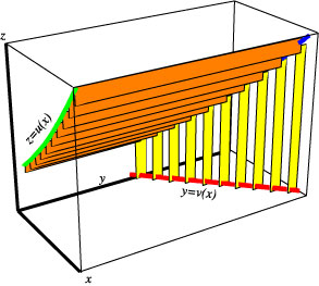
    The integral is the limit of the sum as tends to infinity and the norm of the partition   of the interval [a,b] tends to 0, taken over all choices of the numbers . Note again that under our assumptions on and , this definition is compatible with the definition of the Riemann integral (when is viewed as the Riemann integral ). The sum    can be interpreted as a sum of areas of the (yellow) vertical rectangles in Picture 1.

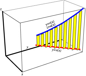
Picture 1.

    Zoom in to notice a few features of the image that we will need later.

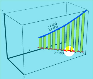Picture 2.

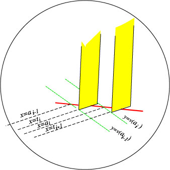Picture 3.

    We see in the last image that the (yellow) vertical rectangles are all parallel to the yz-plane and that their orthogonal projections on the yz-plane do not overlap.

    Now we do the same visualization of the Riemann/Riemann-Stieltjes sums corresponding to the integral  . For reason that will be apparent below, we now interchange the roles of the y and z axes.

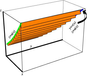
Picture 4.

    Here is an amalgamation of the images 1 and 4.

Picture 5.

    We rotate this object to get a view of its orthogonal projection onto the yz-plane. In the animation below we take a finer subdivision of the interval [a,b] so that the sums   and   give better approximations of the integrals and respectively. (Please press and hold the control key and then click on the image to play the animation or press the right mouse key and then click on the "play" option)

Picture 6 (Animation)

 Let us pay attention to the last frame where we see the projection of the rectangles and the curves onto the yz-plane (somewhat off the desired orthogonal projection because of the perspective). As observed above (Picture 3), we do not lose anything of the total area of the rectangles in that projection.

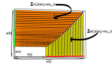
Picture 7.

    We see that   + is approximately equal to and (*) follows by taking the limit as .