Name: Anthony B. Davis, PhD, Physicist (b. Montréal, Québec, Canada, 1952). 

Address: Space & Remote Sensing Sciences Group (NIS-2), Los Alamos National Laboratory, P.O. Box 1663 (MS C-323), Los Alamos, NM 87545, USA. 

E-mail: adavis@lanl.gov

Fields of interest: Mathematical geophysics, fractal geometry, multifractal statistics, three-dimensional radiative transfer theory, remote sensing, clouds, extreme atmospheric phenomena, environmental policy and security concerns (music, films, travel, history).

Awards: Performance Award, NASA’s Space Flight Center 1997; Performance Award, Los Alamos National Laboratory 1999.

Publications and/or Exhibitions: Davis, A. B., Reeves, N. M., and Cahalan, R. F. (1995) Architecture of clouds - clouds as architecture, scale-invariance as a symmetry in natural systems and artificial environments, In: Darvas, G., and Nagy, D., eds., Proceedings of 3rd Interdisciplinary Symmetry Congress and Exhibition "Symmetry: Artificial and Natural," August 14-20, 1995, Washington (DC), published in Symmetry: Culture and Science, Vol. 6, No. 1, 137-140.
 

Abstract: Wavelets are the mathematical equivalent of a microscope, a means of looking at more or less detail in data. By applying wavelet transforms to remote sensing data (satellite images, atmospheric profiles, etc.), we can discover symmetries in Nature’s ways of changing in time and displaying a highly variable environment at any given time. These symmetries are not exact but statistical. The most intriguing one is "scale-invariance" which describes how spatial statistics collected over a wide range of scales (using wavelets) follow simple power laws with respect to the scale parameter. The geometrical counterparts of statistical scale-invariance are the random fractals so often observed in Nature. This wavelet-based exploration of natural symmetry will be illustrated with clouds.
 

1 WAVELET TRANSFORMS

Consider some geophysical variable of interest f, dependent on position in space or time x, that we will denote f(x); this is nothing more than a long string of numbers obtained from an instrument or a model calculation. The general philosophy of wavelet analysis is the separation of this signal into a slowly varying, or "local average," part and the remaining fast-varying part, or "fluctuation." In fact, this is often a goal in life generally speaking: how to separate the big-picture from the details, the forest from the trees, etc? Mathematically, this separation corresponds to two complementary filtering operations. A wavelet filter looks like this
 

(1) 

We use a to denote the scale at which we separate the "fast" and "slow" components and b as a position parameter. The mathematical shorthand in Eq. (1) is now translated into plain language.

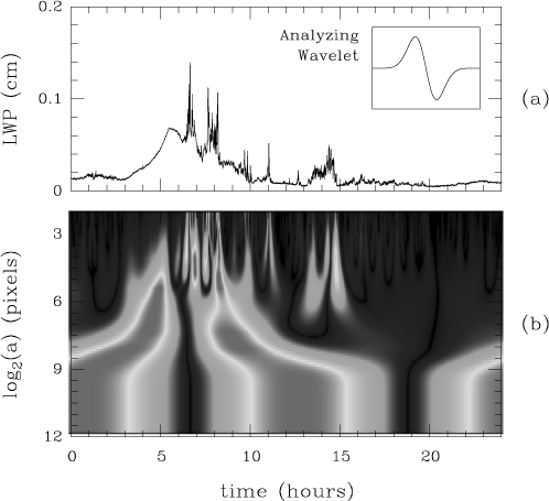
The function y(x) is the so-called "mother wavelet" that it is only required to have a vanishing mean value, hence to oscillate at least once around zero; it is usually assumed to take (significantly) non-vanishing values only near or around the origin x = 0. Thus, the term ya,b(x) in the above equations is a dilated (a > 1) or shrunken (a < 1) version of the mother wavelet form that is also displaced by a distance b in either direction , to the right (b > 0), or to the left (b < 0). Notice the built-in connection with zoom- and displacement-transforms respectively. The integral operation on the r.-h. side of Eq. (1) just means ‘form the product of the (scaled/shifted) wavelet and the input signal, then sum over all (available) values of space (or time).’ The result is an "image" of f(x) through the wavelet transformation (WT), based on a certain choice for y(x), that will depend on a and b. So the notation Ty[f](a,b) on the l.-h. side represents a 2D array of numbers resulting from the operation prescribed on the r.-h. side, with a book-keeping of sorts for all the dependencies it inherits.

If the local mean is the desired outcome at scale a, rather than the fluctuation, then one uses a "scaling function" j(x) rather than a wavelet y(x). The only difference is that it does not need to oscillate or, more precisely, it should have a non-vanishing mean. Otherwise, the same notation applies: Tj[f](a,b), just as in Eq. (1).

Figure 1 shows the image of a specific function f(x) though a specific WT. The graph of f(x) is plotted in the top panel (a); it is a trace in time of the amount of liquid water in the cloudy atmospheric column above a instrument station in Oklahoma for one day; sampling is done every 20 seconds. The two-dimensional result from Eq. (1), Ty[f](a,b), is illustrated in the lower panel (b) on a grey scale in absolute value, denoted |Ty[f](a,b)| in the following; note that the scale parameter a increases downward. The choice of analysing wavelet is shown in the inset in panel (a).
 
 

2 STATISTICAL SCALE-INVARIANCE

In observations of geophysical fields or time-series, there are two operationally important length- or time-scales: the total length of the record, L, and the interval between two subsequent samples, l. Thus, the total number of samples in the record is N = L/l where l is the smallest and L the largest scales sampled in this observation (e.g., N = 4320 in Fig. 1). One of the simplest possible spatial statistics to examine is 
 

(2)

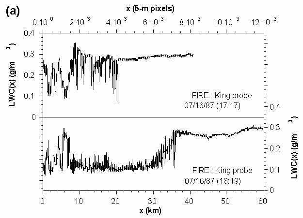
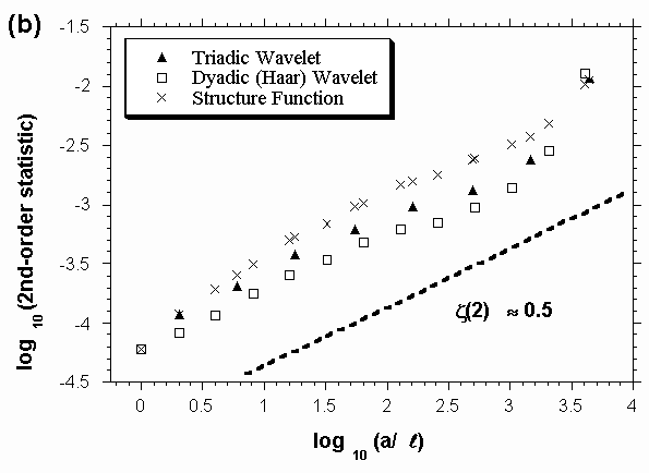
where á·ñX means ‘average the quantity inside the triangular brackets (over the variable(s) in the sub-index).’ So Sy(q;a) is just the qth-order statistical moment of the absolute y-WT coefficients at scale a. In this case, we have averaged over all positions (b-values in WT) and, if possible, over all the different "realisations" of the random signal f. If the data is scale-invariant (with respect to zoom operations), then it can be shown that Sy(q;a) must be a simple power-law function of a as indicated on the r.-h. side of Eq. (2) where "µ" means ‘proportional to.’

Figure 2a shows typical data on internal cloud structure from long aircraft penetrations into marine stratocumulus layers. Such persistent and extensive clouds form almost daily off the coast of California and off other Eastern shores of the world’s oceans. Because of their ubiquity and strong reflectivity, these clouds are an important factor in the Earth’s climate. From there, we can understand the need to better characterise their internal structure; their outer structure is not very interesting: essentially, flat top and base. The data is "liquid water content" (LWC) which measures (in g/m3) the amount of water contained in the droplets suspended in the cloudy air sampled by a special probe under the wing of an aircraft every 5 meters along the horizontal flight path.

Figure 2b shows log10Sy(2;a) versus log10a for three different choices of the analysing wavelet y, including a "poor-man’s wavelet" consisting of just the difference between two LWC points separated by a variable distance a: Ty[f](a,b) = f(b+a)–f(b) and Sy(2;a) = á| f(b+a)–f(b)|2ñb,f. This older approach in data analysis restricted to q = 2 is known as "structure functions" (Monin and Yaglom, 1975) or the "semi-variogram" (Christakos, 1992; and references therein). The tendency of the statistical results to align rather well in the log-log plot shows that scale-invariance prevails, as defined by the power law in Eq. (2). So, in spite of its appearance in Fig. 2a, LWC data has a hidden symmetry, that of scale-invariance. We also note that the exponent zy(2), defined in practice as the slope of the line in Fig. 2b, is not very sensitive to the choice of wavelet; for more information on why/when this is expected and not, we refer the interested reader to the review article by Muzy, Bacry, and Arnéodo (1994).

References

Christakos, G. (1992) Random Fields in Earth Sciences, San Diego, Calif.: Academic Press, 474 pp.

Monin, A. S. and Yaglom, A. M. (1975) Statistical Fluid Mechanics, Vol. 2, Cambridge: MIT Press, 683 pp.

Muzy, J.–F., Bacry, E., and Arnéodo, A. (1994) The multifractal formalism revisited with wavelets, International Journal of Bifurcation and Chaos, 4, 245-302.