Turk’s-head knotS
(BRAIDED BAND KNOTS)
A Mathematical Modeling
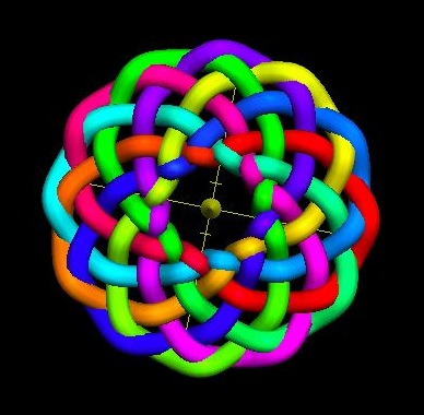
Figure 1
A 12-Bight, 7-Lead, Single-Ply Disk-Shaped Turk’s-Head Knot
To be respectful, first of all, I should say a word about the nomenclature, “Turk’s-Head” knots, for were I of Turkish descent, I might be offended by the term:
The name first appeared in the knot literature in Darcy Lever’s 1808 book, The Sheet Anchor , according to Clifford W. Ashley, in his 1944 comprehensive and unequaled to date publication, The Ashley Book of Knots . I have heard nothing quoting an earlier date of first publication of the term. Ashley goes on, amending Lever and saying, “This resemblance to a [Crown or] Turban presumably is responsible for the name ‘Turk’s-Head,’” and furthermore, “There is no knot with a wider field of usefulness.”
These Disk-Shaped (See Figure 1 ) or Tubular (See Figure 2 ) Alternating knots are now known almost universally by the name, from Great Britain to Japan. Perhaps if up to me, I might call them Braided Bands or Braided Rings.
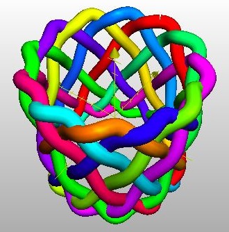
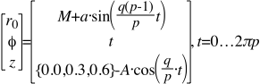
Figure 2, Above.
Tubular, or, Cylinder-Shaped Knot of 12 Bights & 7 Leads.
(The Outside rim of the Disk shaped knot has become the Top of this Tubular one.)
Usually, when a sailor refers simply to a “Turk’s-Head” knot, in general, he is referring to a Single-Piece Common or Running one. This is, as opposed to a Fixed or Standing Turk’s-Head knot which is tied of multiple pieces of line and is spliced into something such as the case for a footrope or manrope hold, or onto something such as for the case of coxcombing onto a stanchion.
The family of Single Piece, Common Turk’s-Head knots is one of the most attractive series of knots ever devised or discovered. Their natural and mathematical beauty is part of the fascination they hold, in addition to their practical, utilitarian functions. They are quite ancient, with representations often found carved in wood, ivory, bone, and stone. For example, they have been found carved into columns within some Egyptian Pharaonic tombs.
As you have seen Figure 1 & Figure 2 , you might be wondering right about now just what is a “Bight” and what is a “Lead” (pronounced “leed”)?
A Bight is a scallop or curve at the rim of of the knot where the cord changes direction.
Given a Common, Running Turk’s-Head knot, there is only one number of Bights, a positive integer. For the case of a flat disk-shaped knot, if you count (as a person often has to do), the number is the same around the inside hole as around the outside rim of the disk. For the case of a tubular cylindrical knot the number at the top of the tube always equals the number at the bottom.
A Lead is a single path or revolution of the cord around the tubular band, or if a flat knot, around the hole in the center of the disk, while discounting the extra “parallel” threading or following of the original knot when an extra Ply or two is put into the knot. (For a little confusing terminology and tradition, sailors call putting an extra ply or two into a knot, “doubling” and “tripling,” or, “doubling twice.”) I will try to keep such confusing lingo to a minimum in this article.
Given a common Turk’s-Head knot, there is only one number of Leads, a positive integer, which happens to be equal to Two or greater, because after all a knot of only one Lead would be the Unknot.
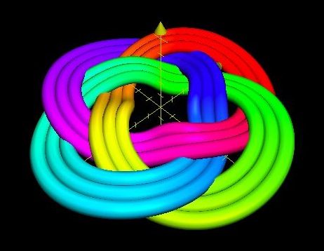
Figure 3, Above.
This knot has 4 Bights & still only 3 Leads, although shown 3-Ply.
The cord goes over three & under three, in its weaving around the knot.
By tightening some parts and loosening of others, a tubular cylinder-shaped Turk’s-Head knot may be manipulated by hand into a flat disk-shaped knot, and vice-versa, while preserving the number of bights and the number of leads.
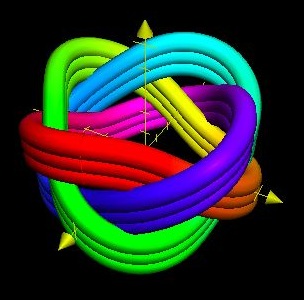
Figure 4, Above.
A Cylindrical Turk’s-Head Knot of 4-Bights & 3-Leads--The represented actual
tubular knot may be changed to or from the actual knot represented by Figure 3.
(The Top of this Tubular knot is the Outside of the Disk knot.)
Furthermore, Common Turk’s-Head knots are Alternating Knots, with a regular over one, under one weave, or an over two, under two weave, or an over three, under three weave and so on. This is sometimes referred to as a “Basket” type of weave. The parallel extra plies put into the knot preserve the underlying structure of the original One-ply knot.
Figure 3 & Figure 4 illustrate the last two mentioned properties.
In this article, I will frequently jump from Disk-shaped models to Tubular Cylindrical models, and back again, in layers of complexity. This article, and the models, cannot be summed up in a one sentence “sound bite.”
The three-dimensional Cylindrical Coordinate graphing system lends itself particularly well to mathematically modeling Turk’s-Head knots, because Turk’s-Head knots are usually either (1) circular disk-shaped flat knots, or (2) cylinder-shaped 3-D knots.
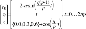
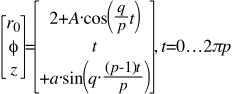
Herein, in Cylindrical Coordinates, Position is given by an independent variable, t in these cases, which the Angle Phi ϕ takes on, and a Radius r 0 and Height z , both of which are functions of t .
Using Radians to measure angles (There are 2π Radians for every 360 Degrees.), the modeling equations utilized to produce the Figure 1 Disk shaped Turk’s-Head knot, in Cylindrical Coordinates, are:
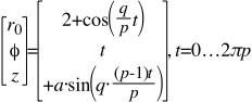
Where q = 12 Bights, and p = 7 Leads
And a = 0.25 = amplitude of the Sine function in this case, which gives the maximum Height or depth from the plane of the Disk, as the cord weaves up and down. Thus, (a) roughly speaking equals the diameter of the Cord used to tie the knot.
These three equations are not as complex as they may seem at first, when they are broken down into their component parts:
If the Radius, r 0 were to = a Constant (in this case, a Midrange Radius = 2 units), then we would have the equation for a Circle.
If an appropriate wave, such as a Cosine wave, is added to the Circle, then we will have a wavy, braided graph with the right number of Bights and the right number of Leads.
A Cosine wave is chosen, because a cosine wave will have a maximum at its starting point of t = 0 radians.
The Cosine wave will have to go around (p) times, because there are (p) Leads, and therefore (2πp Radians) is the upper limit for (t) , before the graph will start repeating itself.
This Cosine wave is the essence of the model, as the cord undulates from an outside bight (where the cosine function = +1) of the Disk, to an inside bight (where the cosine function = -1). The total Disk Diameter is 6 units, figured as twice the maximum radius of (2+1).
As far as the (z) thin height of the Disk-shaped knot is concerned, the Number of Intersections, or Crossings, is figured as equal to (q)(p-1), that is to say, there will be at least one intersection for every Bight and for every Lead minus one, since the width of the braid is #Leads wide.
This number, ((q)(p-1)) , is the total number of periods for the thin height Sine wave function.
Since the number of times the wavy, braided graph must go around is ( p ) times because there are (p) Leads, we have the fraction of ((q)(p-1)÷(p)) for the height Sine wave function, and as mentioned above, an amplitude of (a).
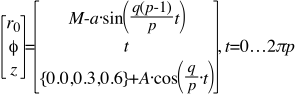
In Cylindrical Coordinates, the modeling equations utilized to produce the Figure 2 Cylinder-or Tubula r shaped Turk’s-Head knot are:
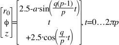
Again, q = 12 Bights, and p = 7 Leads.
However, for the Tubular model this time, the cord weaves in and out from a given Midrange Radius (= 2.5 units) of a Cylindrical surface, instead of crossing up and down from a plane of a Disk.
A thin Sine function is used, as a = 0.25 units = cord diameter.
Please Note :
The Sine expression is preceded by a Minus Sign, because the outside rim Top of the Disk knot has become the Inside top lip of the Tubular knot. The cord must weave Inward (negatively) for the Tubular knot at points where the cord has woven upward (positively) in the Disk .
Because this cylinder-shaped knot has a Midrange Radius of 2.5 units, its Diameter across is (5.0 + 2a ) units.
More significantly, it is the Height along the z- axis which uses the Cosine function, as the cord undulates from a high bight to a low one. The Height will vary between (+2.5 units) and (-2.5 units), and therefore total (5.0 units).
The twice appearing numbers “2.5” are not so important in themselves. They are merely scalar quantities. What is important, in this case, is that they do appear twice, giving Relative values to each other such that the diameter of the cylindrical knot is roughly equal to its height.
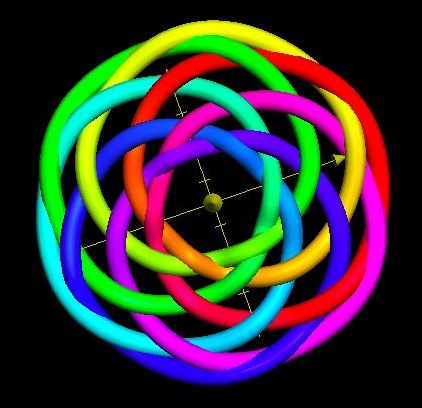
Figure 5, at Left.
q = 6 Bights & p =7 Leads
An example of a “Square” Disk shaped Turk’s-Head knot.
The knot is called “Square” because q (#Bights) & p (#Leads) differ by only 1.
In this case, #Leads > #Bights. The reverse can also occur in a Square Turk’s-Head knot.
Figures 3 & 4 also illustrated a Square Turk’s-Head knot, but for q = 4 Bights and p = 3 Leads.
Because the knots depicted in Figures 3 & 4 have multiple plies, multiple values within braces are added to the Cosine function in each model.
In the Disk knot of Figure 3, the multiple values are Midrange Radii, and are as thus:
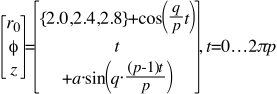
Where q = 4 and p = 3 and a = 0.25
This is about as complicated as it gets. Bear with me here. You’ve made it this far. About all that remains, is to include another, larger Amplitude factor, A , (not to be confused with the smaller a ) with which to multiply by the Cosine expression.
Returning to the Tubular knot depicted in Figure 4 , and which has multiple plies, the modeling equations are:
Again, q = 4 Bights, p = 3 Leads, and a = 0.25
Please notice for this Tubular knot, as with the Disk model, there are multiple values within the braces which are added to the Cosine expression.
And here too, the Cosine expression may be multiplied by an Amplitude factor, A . Also, the Midrange Radius, which above has a value of 2 units, may be replaced with that of another value.
Something that needs mentioning is that in all the models of Common Turk’s-Head knots in this article, and in all known of, the Number of Bights (q), and the Number of Leads (p), must be in their lowest possible relative terms, and may have no common factor (or, “divisor”). The models help explain this phenomenon. If they do, in the models, the factor will cancel out in both the numerators (#Bights, q) and the denominators (#Leads, p). In such a case, the resulting modeled knot will have both fewer Bights and fewer Leads, and it may not form a braided knot at all, but rather the Unknot .
What are some other implications/predictions of the math models? Let’s take a look at another Tubular Turk’s-Head knot in Figures 6 & 7 .
For Figure 6 , the modeling equations (Please notice the Minus & Plus signs preceding the trigonometric expressions) are thus:
q=8 Bights, and p=3 Leads, which is an Odd Number of Leads
M = the Midrange Radius = 2.2 units = 1/2 the diameter of the Tube
A = Amplitude = 1.2 units = 1/2 of the Height of the Tube
a = amplitude of the thin cord diameter = 0.25 units
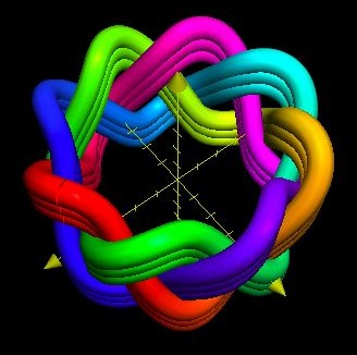
Figure 6 at Left
8 Bights & 3 Leads,
An Odd Number of Leads
Notice the way the cordage spirals up, out, and then down at the top lip of the knot in a Clockwise manner.
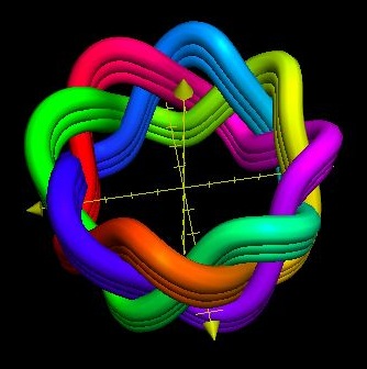
Figure 7, at Right.
8 Bights & 3 Leads
Notice the way the cordage spirals up, out, and then down at the top lip of the knot in a Counterclockwise manner in this case.
This Figure 7 shows the Mirror Image of the above Figure 6.
The Figure 6 knot has been turned inside out to produce the Figure 7 knot. What was the top has become the bottom, and what was formerly the inside has become the outside.
In order to flip a point from the top to the bottom, the Plus sign in front of the Cosine expression becomes a Minus sign. Likewise, for a point on the inside to flip to the outside, the Minus sign in front of the Sine expression changes to a Plus sign.
The modeling equations for Figure 7 therefore become thus:
With the same parameters, as for Figure 6, of M, A, a, q, & p.
The knot is therefore Amphicheiral. By definition of the word, by manipulation the knot may be changed into its mirror image.
This appears to be the case, anecdotally, whenever the Number of Leads (p) is an Odd number. An Odd Number ( p) seems to produce One single knot.
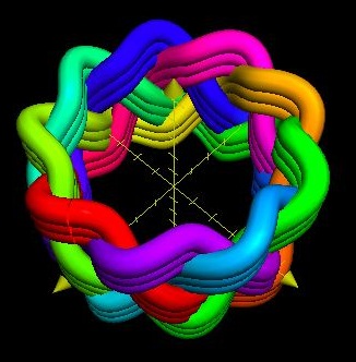
Figure 8, at Left.
9 Bights & 4 Leads,
An Even Number of Leads.
Turning it inside-out, by changing Both signs preceding the trig expressions in the modeling equations, produces the Same image as shown here.
Changing One sign or the other to its opposite will produce the mirror image, but will be a second, different knot, as far as the tying of them can tell.
Utilizing Disk Turk’s-Head knot models apparently yield the same result:
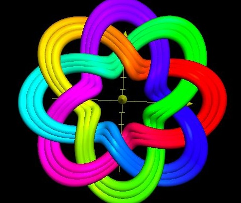
Figure 9, at Right.
8 Bights & 3 Leads
Look at an outer bight and see how it spirals from center outward in a Clockwise manner.
This modeled knot is the same physical knot as the Tubular one shown in Figure 6, but with a Disk set of equations here.
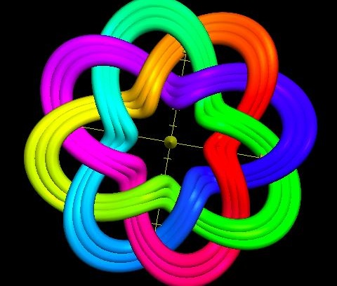
Figure 10, at Left
Also 8 Bights & 3 Leads
This knot Spirals outward at its outer bights in a Counter- clockwise manner.
This graph is obtained by changing, in the Disk equations, Both Plus signs preceding the trigonometric expressions into Minus signs.
The Figure 9 Disk modeling equations are:
Whereas the Figure 10 modeling equations (Notice the Minus signs) are:
In both cases above, q = 8 Bights, p = 3 Leads, and a = 0.25
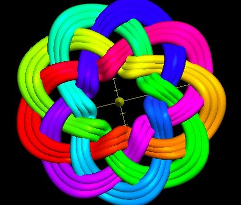
Figure 11, at Left.
9 Bights & 4 Leads,
An Even Number of Leads.
The simple process of turning inside out, by changing the inside to the outside, and the top to bottom (in depth out of the plane of the page), will result in an identical knot.
Amphicheirality, or rather, lack of it, cannot be established by such a simple process in this case.
The equations for the Disk in Figure 11 are the same as for Figures 9 & 10 , but with the obvious difference that q = 9 Bights and p = 4 Leads.
You might be wondering right about now:What about special cases such as the duo of Trefoil (Overhand) knots? Or the special case of the Figure Eight knot (a 2-Bight, 3-Lead Turk’s Head knot)? Or of Two-Lead Torus knots?
Do the mathematical models hold for these special (minimalist) cases? The answer appears to be Yes.
One special case was touched upon way back in Figure 3 The knot depicted there was the 4-Bight, 3-Lead special case which is so common that it also goes by another name, a “Sailor’s Breastplate” knot. However, the actual tied knot, of which Figure 3 is a depiction, will have two ends to the piece of rope. In the actual 3-Ply knot, after one cord end has worked its way around three times in order to make it 3-Ply, the ends do not match up directly to touch each other. Usually, in such an actual case, the cord/rope ends are whipped and then seized into place with marlin on the under side of the knot, where they will not show from above.
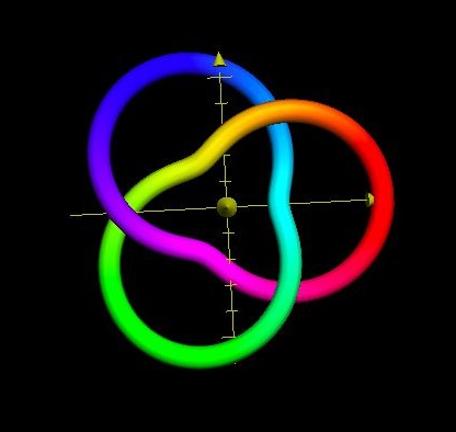
Figure 12, Above.
This is a Trefoil (Overhand) knot using a Disk Model;
A special simple case:
It is a 3 Bight, 2 Lead Turk’s-Head knot,
And also a (3,2) Torus knot.
The Trefoil knot is actually two knots. There is one, as in Figure 12, in which the cordage spirals out, at its outside bights, in a Clockwise manner; There is a second Trefoil with a Counterclockwise manner, which may be modeled by changing one, but not both, of the Plus signs in front of the trig functions, into a Minus sign..
Modeling Cylindrically, the Figure 12 Trefoil knot looks something like this:
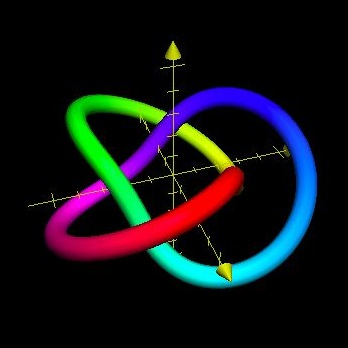
Figure 13, Above.
The previous knot, shown here Cylindrically;
The Overhand knot is distinctly visible,
on the left side of the figure.
The Figure Eight knot can actually be modeled by a 2-Bight, 3-Lead Turk’s-Head knot.
Additionally, one modeled Figure Eight knot may be changed to its mirror image by turning inside-out.
Knot tyers sometimes call the process of changing a knot into its mirror image, “flyping” the knot.
They can look something like the following two figures.
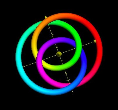
Figure 14, at Right.
2 Bights & 3 Leads
A Figure Eight Knot
Try tying the knot as shown. You will see it actually is a Figure Eight knot!
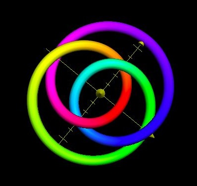
Figure 15, at Left.
2 Bights & 3 Leads
The same Figure Eight knot as shown in Figure 14, but turned inside-out, producing its mirror image.
Thus, there is only one Figure Eight knot.
Finally, we come to the special simple cases of 2-Lead Torus knots. Because the number of Leads is so low as to equal 2, these Torus knots should have equivalent output graphs as 2-Lead Turk’s-Head knots. The number of Bights (q) must be an odd Cardinal number, since the number of Leads (p) is an even number..
Take a random odd Number of Bights, say q=9. A Disk modeled graph might look like this:
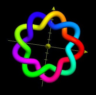
Figure 16, Above.
Where:
And where: A=0.5, a=0.25, and q=9 and p=2
The Disk Model appears to hold in this special simple case, as well. A 3D Cylindrical Model of the (9,2) Torus produces a similar result.
Because the models in this article involve periodic cosine & sine functions, you might be wondering, what specific periods, or, wavelengths are involved? Remembering there are 2π radians for every 360°, the periods may be briefly summarized as follows:
For the entire Turk’s-Head knot: 2πp radians
In a Disk shaped knot, from one outside bight to the next outside bight: (2πp/q) radians
In a Cylindrical knot, from one top bight to the next top bight: (2πp/q) radians
In a Disk shaped knot, from one outside bight to the next inside bight: (πp/q) radians
In a Cylindrical knot, from one top bight to the next bottom bight: (πp/q) radians
From one over (under) crossing to the next over (under) crossing: 2πp/(q(p-1)) radians
From one crossing to the next crossing: πp/(q(p-1)) radians
This brings us back to the rather central question: Why model Turk’s-Head, or Braided Band, knots in the first place?
As you have seen, the knots are quite handsome. Their sheer beauty is reason enough. Besides which, they are fun to model. And thirdly, simple graphical models or aids are often utilized in order to be able to tie some Turk’s-Head knots in the first place. Then the knots may be applied for ornamental or practical purposes.
Often, something is not fully understood until a model is made of it, whether the model be a physical one such as a scale model, or a mathematical model, or a graphical model, or some other type.
I believe the models, such as in this article, may simulate any Common Turk’s-Head knot that is possible to be tied, within practicable limits. These periodic models may prove to be valuable if they are generalized to other applications. Hopefully, good will come from them.
It seems that just about any kind of theoretical mathematics, like any innovation, sooner or later becomes applied to practical purposes. Perhaps the application occurs so readily, because the theoretical is inspired, or has a taking off point, from that which is observable.
Why model knots? Why? Why Knot?
To tie a knot utilizing one of the Disk models, you will need a printout (reduced or enlarged to full size, usually by photocopying), round-head quilting pins (or nails), and a craft board (or a piece of wood or plywood). The pins (or nails) are used for guideposts to weave around and not to pin down the cordage. First you will need to make a measurement single pass of the cordage around all or some of the knot’s revolutions. This measurement also tests the pin (nail) locations as guideposts. The sized printout shows you where to weave under, where to weave over, and what direction the rope, cord, or string should take. It is that simple.
To tie a tubular Turk’s-Head knot from a model, First tie a one-ply Disk knot. Then, remove it from the pins (or nails) & craft board and fashion it into a cylindrical shape by hand. Add extra plies as desired. Then draw up the knot, tight and even as needed.
* * *
The author would like to thank Dr. Slavik Jablan for his support and encouragement, expertise and efforts which make possible publication in VisMath .
The author would like to thank Rosalyn R. Carpenter and Thomas M. Hughes for their assistance and support in proofreading and readability of this article.
The author would like to thank Anne W. Pennock for the unwavering support that made this article possible.
The author is indebted to the folks at Apple Computers who offered as standard software, the “Grapher,” that is, a graphing calculator package. This includes the mathematical equations for a Torus knot Grapher Example, which was invaluable as a starting point.
The author would like to cite the following two texts as sources:
Adams, Colin C., The KNOT book, An Elementary Introduction to the Mathematical Theory of Knots , W.H. Freeman and Company, New York, New York, 2001. This book was given to the article’s author by Phyllis J. Robinson.
Ashley, Clifford W., The Ashley Book of Knots , Doubleday & Company, Inc., Garden City, New York, 1944. A copy of this book was given to the author by Wallace McCurdy and Family, including Martha.
Skip Pennock, Monday, 12 September, 2005
Member, The International Guild of Knot Tyers (The IGKT)
The IGKT Website: www.igkt.net
The author is not a mathematician by trade, but rather an artist/craftsman. Over the course of two dozen years, he has designed/discovered/rediscovered several thousand new, primarily two-dimensional, flat knots in hundreds of different shapes & silhouettes.
Published material by the author includes a craft book, Decorative Woven Flat Knots , published by The IGKT in 2002, and since, a couple of articles pertinent to Turk’s-Head knots, or, Braided Band knots.
This includes an article published in VisMath , the Journal of ISIS Symmetry: Volume 6, No. 4, 2004, Article No. 4.