|
Frustration, Degeneracy and Forms A View of the Antiferromagnetic
Tohru OGAWA1) and Yukihisa
NAKAJIMA2)
1) Institute of Applied
Physics, University of Tsukuba, Ibaraki 305,
2) Office of Statistics,
Japan Meteorological Agency, Ohtemachi, Chiyoda-ku, Tokyo 100
Some
exchange kinetics are introduced into the antiferromagnetic Ising model
on a triangular lattice. These connect the degenerate ground-states and
give rise to a set of random walks over the resulting irregular network
in the phase space. Some theoretical analysis of the elementary processes
is presented together with the results of a related Monte Carlo experiment.
Some features of the system are found suggestive of a liquid-glass transition,
although we have not yet conclusively demonstrated the existence of such
a transition in this system. An approximate ground-state energy is also
evaluated for the antiferromagnetic Heisenberg model on a triangular lattice.
1. Introduction An important role of fundamental science is to prepare some views and concepts which are available in extending the scope of science. The attempt in this paper is based on this philosophy [1]. Cellular automata [2] are often studied from a similar point of view, in which simple basic laws governing local processes give rise to highly complex phenomena. These studies are very important in the extension of physical science in the future even though the correspondence with the real physical world may be at most metaphorical or suggestive. For further development along this line, it is desirable to try to include some conservation laws and frustration phenomena in models of cellular automata. A frustrated system is very interesting and important from this point of view because of abundance of states and phenomena appearing in it. We may bear in mind that, in living organisms, a wide variety of phenomena are contained within a very narrow energy range. We may expect the study of a frustrated system to provide an insight into more complex systems than treated hitherto. The cellular automaton models are usually deterministic. However it is very difficult to construct a purely deterministic model with conservation and frustration. Therefore a kinetic model containing stochastic (probabilistic) terms is studied in this paper. The antiferromagnetic Ising model on a triangular lattice is typical of such systems. The frustration produces a degeneracy of the ground-state. The number of degrees of freedom of the ground-states is e0.3231 = 1.381 per site. The residual entropy of the system, which was rigorously calculated by Wannier [3], is proportional to the logarithm of this value. Almost nothing is known of the details of the degenerate ground-states. Some years ago, the author studied their cluster structure [1,4] in relation to some maze-like patterns observed in the monodispersive latex system in a (2+ e)-dimensional space [5]. Though the present investigation [6] is on similar lines, its purpose is more abstract. It is the so-called "glass transition" that is the closest physical effect to the present research. It is supposed that there is no essential difference between a liquid and a glass so far as their static structures are concerned. Or, at least, no abrupt change in the static structure can be expected. The difference in structure between a liquid and a glass may be expected to lie in the dynamics of their phase spaces. If so, the present model is the simplest one that can be investigated in detail. Though the results obtained so far are not enough to draw firm conclusions in this respect, some interesting and suggestive features of this system have been found and are described in the following sections. As a byproduct
of the present formulation, an approximate ground-state energy is evaluated
for the antiferromagnetic Heisenberg model of S=112 on a triangular
lattice.
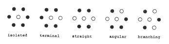
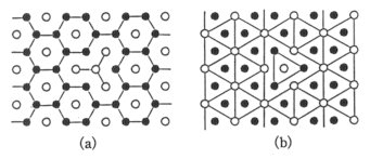
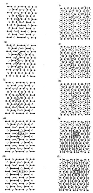
2. A model 2.1. Ground-state ensemble Let us take an antiferromagnetic Ising model on a triangular lattice. Each site takes either of two states, U ("up") or D ("down"). Suppose the number of lattice sites is L and then that of nearest-neighbour pairs is 3L. A basic cell is defined as a regular triangle consisting of three sites which are mutual nearest-neighbours. The number of such basic cells is 2L. Let us confine our attention to a set of configurations which belong to the degenerate ground-state. It may be referred to as the "ground-state ensemble". In fact no energy variable actually enters the following discussion at all except in Section 6. In any member of the ground-state ensemble, it is easily seen that, of the three sites in a basic cell, two must be in one state and the third in the other. This constraint, which is hereinafter referred to as the "basic constraint", characterizes the ensemble. A cluster is defined as the set of the connected sites which are in the same state. For a site in one state, the configuration of its six neighbours is restricted to one of five types, isolated, terminal, straight, angular and branching, shown in Fig. 1. The classification is based on the status of the site in the cluster of which it is a member. The ground-state
ensemble is divided into sub-ensembles according to the value of the specific
magnetization m. This is the difference between the density of the majority
spin state and that of the minority. Without loos of generality, we may
suppose that U state is of the majority, and that the magnetization lies
in the range 0 < m < 1/3.
Two symbols O and · denote either ( O = U, · = D ) or ( O = D, · = U ). The naming is based on the status in the cluster of the central site.
2.2. Graphical representations Some graphical
representation is helpful in illustrating the character of a configuration.
Two representations are given below. The first one is applicable not only
for the ground-states but also for the excited states. The second one is
only applicable for the ground-states.
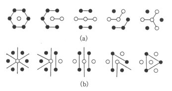
(1) Frustrated-Bond Representation (FB-graph) Join all the neighbouring pairs in the same state by coloured line segments, distinguishing two kinds of states by two colours. They correspond to the frustrated pairs which are in the same state against the antiferromagnetic interaction. Their total length is a constant since exactly one third of all the nearest-neighbour pairs are frustrated. Furthermore, the total length of U-lines is 3(1 + m)L/2 and that of D-lines 3(1 - m)L/2. A set of connected sites in this representation is simply a cluster as previously defined (see Fig. 2(a)).
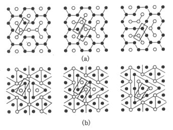
Fig.
2. The five configurations of seven sites shown in Fig.
1 are
(2) Contour Representation (C-graph) Consider a frustrated pair. It is a side common to two basic cells. There are two other sites in these cells. They, being mutually second-neighbour pair belonging to the same sublattice, are in the same state by the basic constraint in the ground-states. In the contour representation, such a second-neighbour pair is joined with a coloured line-segment instead of the frustrated pairs. Therefore the two representations are mutually dual in a certain sense (see Fig. 2(b)). The number of segments which meet at a site is either 0, 2, 4 or 6. It means that any connected figure consisting of such segments is closed and unicursal. This fact is important in the subsequent arguments. The angle formed by adjacent two segments is either 60o or 180o. The colour should be chosen to be one of six depending on the sub-lattice concerned and on the current state. The six colours correspond to (1) a-U, (2) b-D, (3) g-U, (4) a-D, (5) b-U, and (6) g-D. It may also be noted that the colour of the line next to a given coloured line can be one of only two colours. For example, only a-U or g-U can be next to b-D. The integers in the parentheses above, which may be referred to as colour rank, can be used to specify the varieties of line segments instead of the six colours. It is convenient to define the integer in an infinite range and the colours in cyclic in modulo 6 as (7) a-U, (8) b-D, ... If the colour rank is regarded as a digitized "height", then a configuration can be viewed as a topography. Then the coloured lines correspond to height contours. This is the reason why the representation is referred to as Contour representation. This topographical view is very suggestive in predicting what kind of change can take place in the immediate future (see Section 4). When a
periodic boundary condition is imposed, caution is required. If the period
is not an integral multiple of 3, three sublattices are connected by the
boundary condition and cannot be coloured self-consistently. It may be
noted that, even if it is of the form 3n, there is the possibility
that the same colours corresponding to the different heights (which differ
by a multiple of the fundamental period 6) are connected. We may note that
such a "twist" is conserved in a kinetic model to be introduced later.
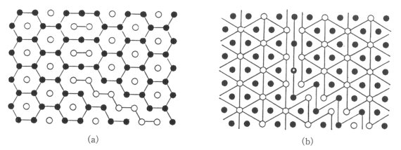
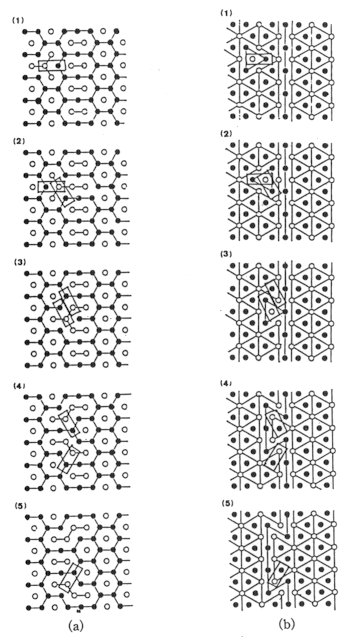
Fig.
3. A boundary between two crystals is represented (a) in the FB-graph
and
2.3. Configurations The situation when m is exactly 1/3 is described as follows. The whole of one of three triangular sublattices is occupied by D states and the whole of the other two by U states. All the sites in the former are isolated giving a triangular lattice and those in the latter are branching giving a honeycomb lattice. Such a single-crystal-like configuration can be specified by the sublattice of the minority state, simply as an a-, b- or g-crystal. The configurations with m slightly less than 1/3 are polycrystalline like. Each of their crystalline domains is characterized by the sublattice of their minority state. A typical domain boundary is shown in Fig. 3. Generally, a boundary is made up of segments of two types: ladder and steps therein. The configurations
of m~0 can be analyzed with the several concepts and tools to be
introduced later in this paper. Especially, the topographical analogy is
powerful after one is trained.
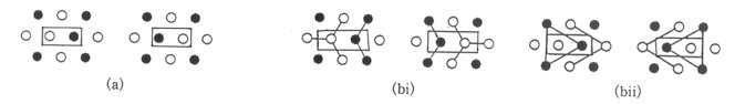
2.4. Kinetic exchange law A kinetic exchange law is now introduced. The states may be exchanged between any nearest-neighbour pair so long as the final state is also one of the ground-states. In other words, the condition for a nearest-neighbour pair to be mobile is as follows. They are in different states and one of them is branching and the other is angular. The condition in the contour representation is simply that a triangle is capped (see Fig. 4). Sometimes a triangle is multiply-capped. Before the introduction of a kinetic law, the ground-state ensemble was merely a simple set as in the conventional equilibrium statistical mechanics. The kinetic law introduces a set of connections between members of the ensemble. The ensemble is now a phase space with a certain topological structure. A kinetic model can be regarded as a random walk in a complicated phase space.
can take place. The pair inside is mobile. (b) The corresponding graphic representations. (i) The FB-graph and (ii) the C-graph.
3. The excitations There
are no mobile pairs for exactly m=1/3, while there are many for
m~0. Suppose the system is an a-crystal and the states U
and D respectively are the majority and the minority.
3.1. A particle A particle-like elementary excitation is defined as follows. A site on a U sublattice, say B, is replaced with the D state and then the replaced site is a branching D-site and their three neighbouring g-sites are all angular U-sites. Therefore the excitation can move in any of three directions. After the motion, it lies on a g-site and can move to one of three neighbouring b-sites. Overall, the excitation can move as a free particle throughout the whole region of the a-crystal. An excitation of this sort is denoted by a Y-symbol connecting the central b- or g-site to neighbouring three a-sites in the FB-graph (Fig. 5(a)) and by a single triangle of side length Ö3 in the C-graph (Fig. 5(b)).
Fig. 5. A particle is (a) Y-shape in the FB-graph and (b) triangular in the C-graph.
Fig.
7. A particle, arriving at a ladder, changes into two steps (more
exactly,
3.2. Two particles Next,
let us study the situation where two particles come close to each other
in an a-crystal. Suppose two particle-like excitations on b have a common
a-site. Then the a-site is a branching D-site and another neighbouring
a-site is an angular U-site. Therefore these two can exchange their
states with each other. The final form seems to consist of three Ls as
shown in Fig. 6. It can be regarded as the smallest
"island" of a b-crystal in an "ocean" of a-crystal.
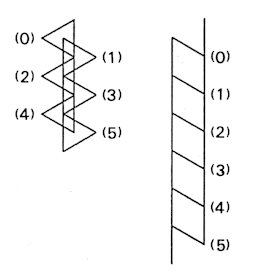
3.3. Steps: excitation of a ladder boundary Suppose a particle in an a-crystal arrives at a ladder-boundary with a b-crystal as shown in Fig. 7. Then two steps are excited on the ladder. The two steps can move independently of each other along the ladder. As shown in Fig. 8, a step moves twice as fast as a particle. In the motion of a step, what is propagated is a pattern (as in a wave). When the steps thus creaed in pairs meet again, they annihilate each other creating a new particle in that crystal from which the original particle came. It can never cross the ladder boundary itself. A remarkable thing is the following: a particle can cross a ladder-boundary with the help of other particles. The situation in such a case is illustrated in Fig. 9. Such an effect is difficult to recognize in the conventional approach.
Fig. 8. A step moves twice as fast as a particle (shown in the C-graph).
Fig.
9. A particle can cross a ladder with the help
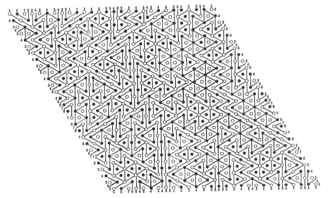
The topographical analogy of the contour graph is very helpful for intuitive comprehension. The C-graph of an a-crystal, is a triangular network of a-D contours with an isolated point of b- or g-site in each mesh. It is analogous to a geographical plain in which low b-hills and shallow g-valleys are periodically arranged. The C-graph of a particle is an isolated hill slightly higher or an isolated valley slightly deeper depending on the sublattice on which it lies. Its motion can be viewed as a meander with its shape alternating between a hill and a valley. A ladder boundary, which is a single straight line in the C-graph, corresponds to a flat slope. A steps-like boundary, being a single zigzag line in she C-graph, corresponds to a hillside with ridges and gullies. Generally, an exchange process is a somersault of a capped triangular contour in the C-graph and rising or sinking in the topographical analogy. After
getting used to this viewpoint, one can acquire some sort of prospect even
for the complicated configurations with m~0 (Fig. 10).
Fig. 10. The C-graph of a configuration with m~0.
5. Monte Carlo experiment A Monte
Carlo experiment was carried out in two stages, using the following routine.
(1) Generation of a gound-state with magnetization m Starting
with any (excited) configuration of U and D of given m,
the following two procedures are repeated until one of the degenerate ground-state
configurations is obtained.
(1a) Sample a nearest-neighbour pair at random.
The Monte Carlo simulation here is essentially a random walk over the network of the phase space. All the microscopic configurations or all the degenerate ground-states should be realized with equal probability. (2a) Sample a nearest-neighbour pair at random. The
reason why a configuration contributes many times in (2c) is demonstrated
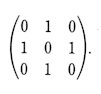
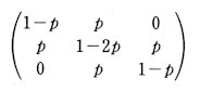
as follows. Consider the simplest case of a random walk on a network consisting
of three points A, B and C where pairs AB and
BC are mutually nearest-neighbour and pair CA is not, as
A-B-C. The matrix showing the neighbouring relation
is given by
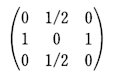
The transition matrix of a related stochastic model
does not give the stationary distribution (1/3, 1/3, 1/3) but (1/4, 1/2, 1/4). The alternative transition matrix
gives the desired stationary distribution for any positive p < 1/2. The latter transition matrix fills the condition of the detailed balance. The situation
can be intuitively understood as follows. A random walker in a city passes
a point on a main street with many crossings more frequently than that
on a bystreet with few crossings if he cannot stay at all. Equality is
happily recovered by putting a staying probability finite. The initial
portions of the Monte Carlo runs should be ignored, since the ground-states
thus obtained lie, so to speak, only at the foot of the "hill" implying
the excited states. The correct averages over equilibrium states are expected
only after a stationary state is realized in the system.
THE MAIN THEME Attention is focussed
on the m-dependence of the following quantities:
(1) The frequency of the exchange processes.
The system
is a 27×27-rhombus region where a rhombic periodic boundary condition
is imposed. In each case, the whole of the first 20,000 (or sometimes 24,000)
movements are ignored under the "birthplace at the foot of the hill"-criterion.
Here, "N movements" means that N exchange processes are actually
observed in the whole 27×27-system. More runs are carried out for
larger values of m, where mobile pairs are rare, in order to get
a sufficient number of independent samples. Then the durations of the runs
are decided in terms of a definite number of movements.
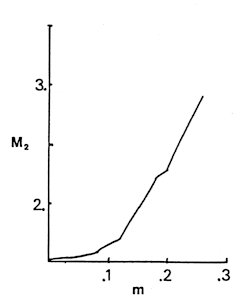
SOME EXPERIMENTAL RESULTS Let Ni
be the frequency with which site i participates in the exchange
processes during 60,000 movements. The second moment M2
of Ni as a distribution over i is shown in Fig.
11. It suggests that a singularity in M2 may exist in
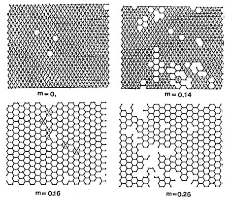
the region m=0.12-0.14. Their spatial distributions are shown in
Fig. 12, where only the sites with Nt > 0.4 Nmax
are plotted as points and the nearest-neighbour pairs among them are joined
with linesegments. It can be seen that the sublattices are not even
in m > 0.14 at least in the time-scale of this observation. This
change in the mode of the movement apparently takes place at 0.14 <
m < 0.16.
Fig.
11. The observed second moment M2 of the frequency
Fig.
12. The spatial distribution of motion for m = O, 0.14, 0.16
and 0.26.
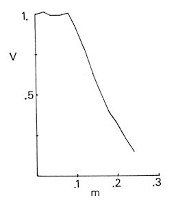
Fig.
13. The unevenness among sublattices that is observed
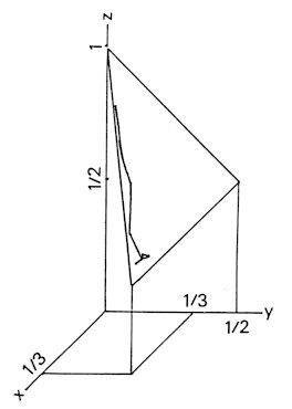
Fig. 14. V=27xyz versus m. Let Fab be the total frequency of the exchange processes between sublattices a and b during 60,000 movements. The quantities X < Y < Z are defined respectively as the maximum, the mediam and the minimum of Fab, Fbg, and Fga. The corresponding normalized quantities x, y and z are defined so that x+y+z=1. Shown in Fig. 13 is the trajectory of the point (x, y, z) for parameter m. The m-dependence can clearly be seen in Figs. 14 and 15, respectively by V=27xyz and by S defined as Ö2 times the area of triangle (x, 0, 0), (0, y, 0) and (0, 0, z). It is noted that V is small whenever x is small and S is small only when both of x and y are small. Remarkably, this is reversed at m~0.08 or 0.10. In the
above, X, Y and Z are defined for F's of the
whole runs. Some trends, however, may exist in the unevenness among sublattices.
Therefore, similar quantities are defined for the time intervals of 8,000
movements. Their m-dependence suggests the existence of some sudden
change at m~0.10.
DEDUCTIONS FROM THE EXPERIMENTAL RESULTS In conclusion,
the Monte Carlo experiment suggests the existence of a big change in the
mode of the exchange processes of the system. However, the singularity
is not so sharp as expected.
In the C-graph, an exchange process produces a somersault of a triangle together with a cap as shown in Fig. 4. The colour of the cap is kept unchanged and that of the triangle changes by ± 2 in colour rank. Nothing else is changed in the system in the respect of the colour scheme. An important
conclusion may be drawn from this result: only by an even number of exchange
processes, can the whole configuration return to its initial state. This
means that the network can be divided into two distinct sublattices. In
other words, the network in the phase space has no frustration even though
the original system has.
APPLICATION TO THE HEISENBERG MODEL The ground-state energy of the antiferromagnetic Heisenberg model on a triangular lattice can be approximately evaluated by making use of the property just mentioned. A Néel state, which is the ground-state of the corresponding Ising model, gives a good approximation for the ground-state in the ordinary system with no frustration. In the frustrated system, the problem should be regarded as that of a perturbation used to resolve a degeneracy. Here, the ground-state is approximated by a linear combination of the degenerate ground-states of the z-component of the Hamiltonian, i.e., that of the corresponding Ising model. Then the diagonalization of the perturbation matrix leads to the ground-state. Note that exactly the same network as in the previous problem corresponds to the transverse component of the Hamiltonian. However, an important difference lies between the two problems: the off-diagonal elements in the present case are connected with the energy while the exchange processes in the previous problem are not [7]. The problem is of the same type as in that of a tightbinding band on an irregular network. The values of all the nonvanishing off-diagonal elements are constant and equal to - J/2>0. The matrix is the same type as Eq. (1). The irregularity is a topological disorder. Because of positive matrix elements, the state of the lowest energy corresponds to the state of the maximum number of nodes. We may remember that the network consists of two sublattices. Therefore the spectral density is symmetrical. Though the ground-state is at the bottom of the band, its properties can be deduced from those at the top of the band, because of the symmetry about the centre of the band. The wave function of the state at the top of the band has no node. If all the coefficients are taken as constant, the expectation value given by the linear combination of the degenerate states provides a lower bound on its absolute value. What is necessary for its evaluation is the number density of the nonvanishing offdiagonal elements. This is equivalent to knowing the probability p that a nearestneighbour pair is mobile in the sense of the previous problem. The ground-states energies are written by E( I ,f ) = - 3 |J| L/4, (4) E( I, af ) = - |J| L/4, (5) E ( H,f ) = - 3|J| L/4, (6) E ( H,af ) = - |J| L/4 - 3 |J| pL, (7) r = E ( H,f )/E ( H,af ) = (1+12p)/3, (8) where I, H, f and af stand for Ising model, Heisenberg model, ferromagnetic and antiferromagnetic, respectively. The argument so far is precise. Unfortunately, however, the estimation of p can now be made only approximately. The subsequent estimation then includes further approximation. Kikuchi's cluster variation method, which was applied in Refs. [1] and [4] to analyze the frequency of the configuration of the seven sites in Fig. 1, gives the value P=0.08, which corresponds to r=0.65. (9)
Acknowledgements The authors would like
to thank Professor R. Collins for critical reading of the manuscript. References
References: [1] The underlying philosophy is mentioned in T. Ogawa, in Topological Disorder in Condensed Matter, ed. F. Yonezawa and T. Ninomiya (Springer, 1983), p. 60. [2] For example, S. Wolfram, Theory and Applications of Cellular Automata*, World Scientific, 1986. [3] G. H. Wannier, Phys. Rev. 79 (1957), 357; B7 (1973), 5017(E). [4] T. Ogawa, J. Phys. Soc. Jpn. Suppl. No. 52 (1983), 167. [5] Y. Koshikiya and S. Hachisu, Lecture at Colloid Symposium of Jpn. (Sept., 1982). [6] Some parts of the present work were reported in Japanese, T. Ogawa and Y. Nakajima, unpublished (Bussei Kenkyu 42 (1984), B30); Proc. Inst. Statist. Math. 33 (1985), 79. Y. Nakajima and T. Ogawa, unpublished (Bussei Kenkyu 44 (1985), B76). Y. Nakajima, unpublished (Bussei Kenkyu 44 (1985), 819). [7] A
relation between a stochastic process and a quantum spin system is discussed
in T. Ogawa, Siiri Kagaku (Mathematical Science) No. 259 (1985), p. 20
(in Japanese).
|
 (2)
(2)  (3)
(3)