|
Fractals and multi layer
Javier Barrallo and Santiago Sanchez Mathematics, Physics and Computer Science The University of the Basque Country School of Architecture. Plaza Onati, 2. 20009 San Sebastián, SPAIN Abstract
Dynamical systems are a well-known branch of mathematics, but until the arrival of computers the sheer number of calculations involved made them impractical for real use. The computers ability to perform rapid calculations allows us to condense billions of calculations into results we can digest. Benoit Mandelbrot was the first one to use computers to produce graphical representations of dynamical systems in the complex plane, based on the quadratic formulas described by the French mathematician Gaston Julia at the beginning of the 20th century. During the 1980s, fractal enthusiasts began exploring fractals for their artistic merit, not for their mathematical significance. While mathematics was the tool, the focus was art. As the fractal equation itself was the most obvious mathematical element, fractal artists experimented with new equations, introducing hundreds of different fractal types. By carefully choosing parameters to refine form, color, and location, these explorers introduced the concept of fractal art. After 1995, few new major fractal types have been introduced.
This is because the newest innovations in fractal art do not come from
changing the fractal equation, but from new ways of coloring the results
of those equations. As these coloring algorithms move from simple to complex,
fractal artists are often returning to the simpler, classical fractal equations.
With the increased flexibility these sophisticated algorithms provide,
there is even more room for personal artistic expression.
2. Coloring algorithms Every dynamical system produces a sequence of values z0, z1, z2 zn. Fractal images are created by producing one of these sequences for each pixel in the image; the coloring algorithm is what interprets this sequence to produce a final color. Typically, the coloring algorithm produces a single value for each pixel. Since color is a three-dimensional space, this one-dimensional value must be expanded to produce a color image. The common method is to create a palette, a sequence of 3D color values; these are connected end-to-end and the coloring algorithm value is then used as a position along this multi-segmented line (the gradient). If the last palette color is connected to the first, a closed, segmented loop is formed and any real value from the coloring algorithm can be mapped to a defined color in the gradient. Gradients are normally linearly interpolated in RGB space (Red, Green, Blue), but they can also be interpolated in HSL space (Hue, Saturation, Lightness) and interpolated with spline curves instead of straight line segments. The selection of the gradient is one of the most critical artistic choices in creating a good fractal image. Color selection can emphasize one part of a fractal image while de-emphasizing others. In extreme cases, two images with the same fractal parameters, but different color schemes will appear totally different. Some coloring algorithms produce discrete values, while
some produce continuous values. Discrete values will produce visible stepping
when used as a gradient position; until recently this was not terribly
important, as the restriction of 8-bit color displays introduced an element
of color stepping in gradients anyway, and discrete coloring values were
mapped to corresponding discrete color in the gradient. With the introduction
of inexpensive 24-bit displays, algorithms which produce continuous values
are becoming more important, as this permits interpolating along the color
gradient to any color precision desired.
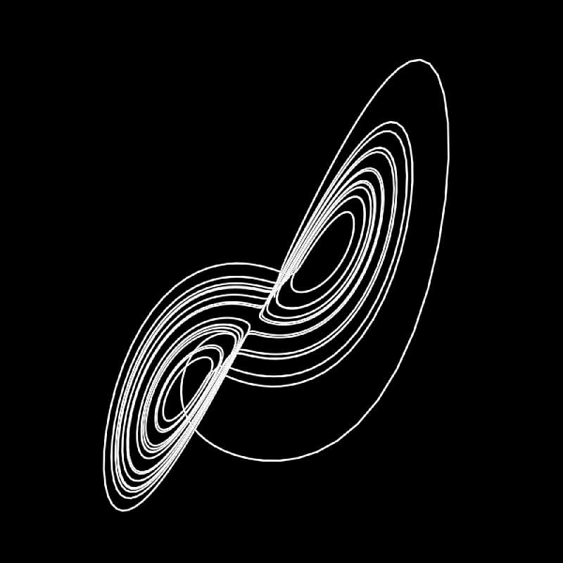
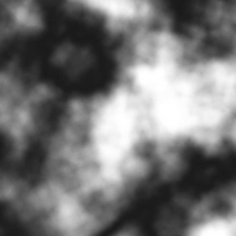
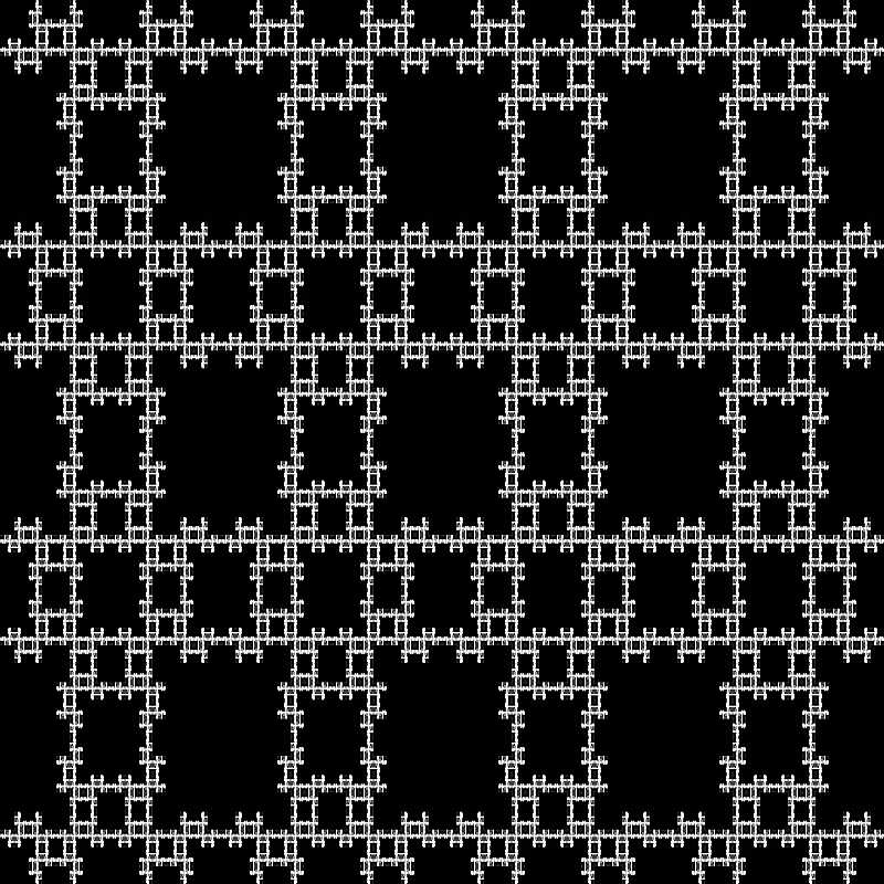
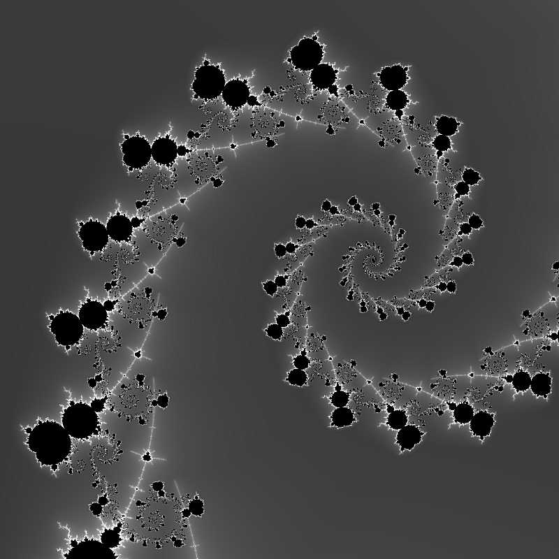
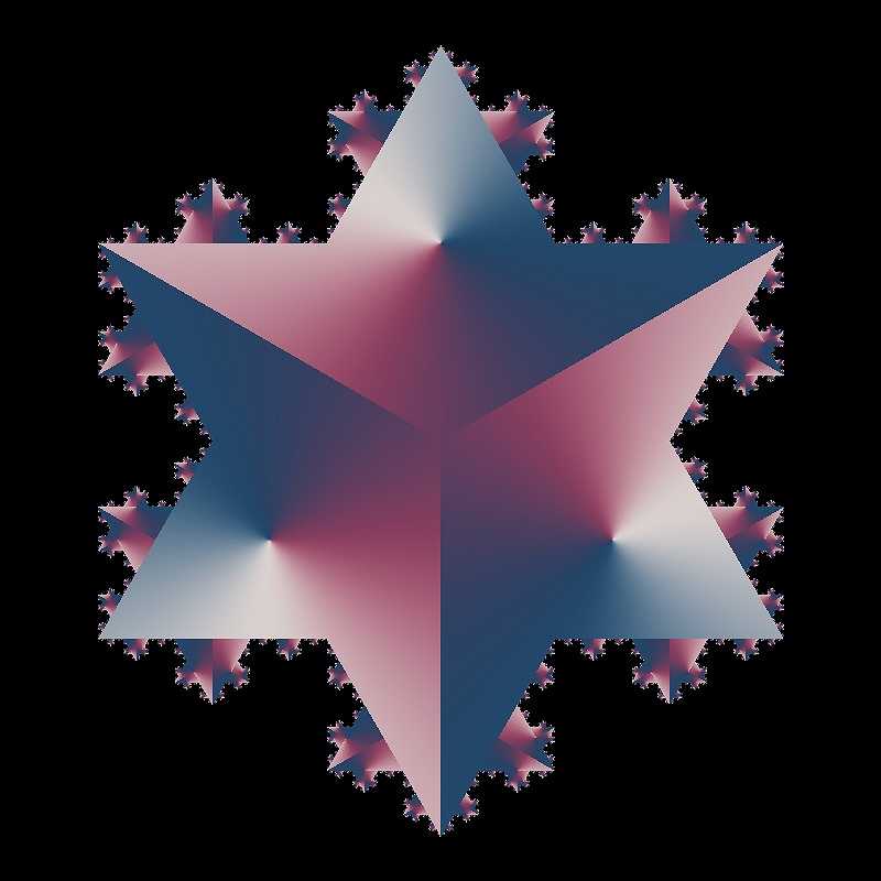
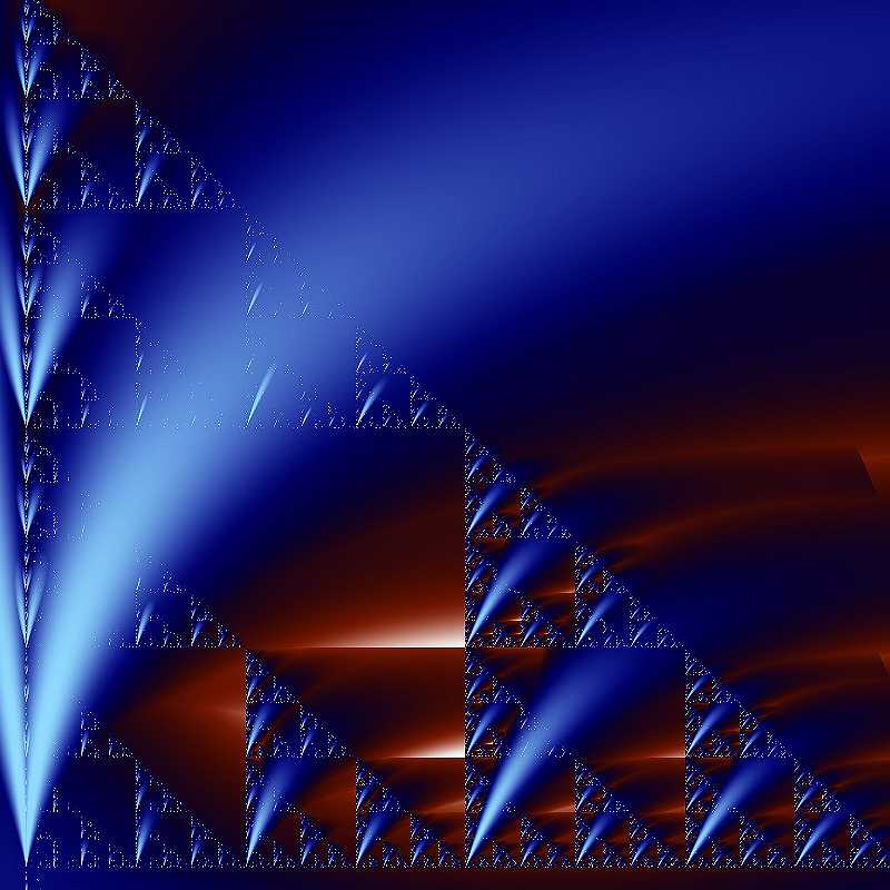
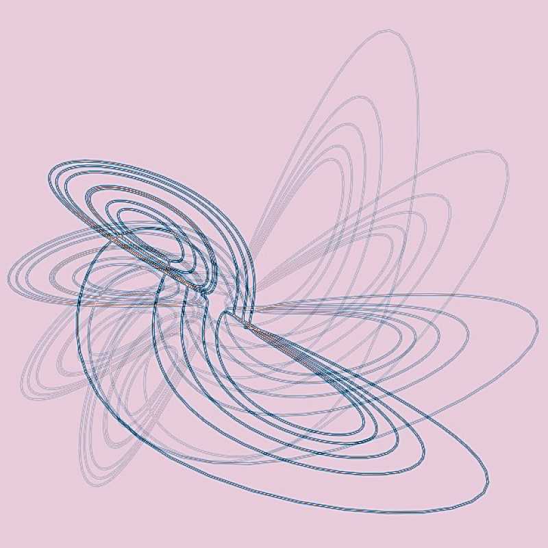
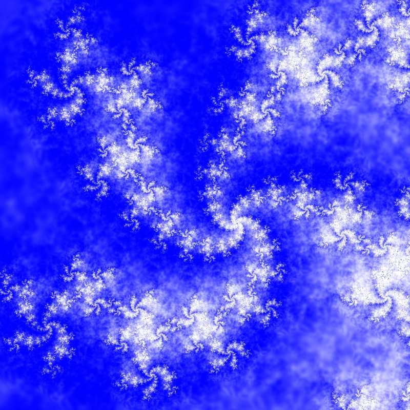
3. Fractal types There are many different fractal types which are not covered when explaining coloring algorithms because they are either not common in fractal explorations or because they are not present in the popular fractal software packages. But basically, we can classify fractal types in six main groups: a) Fractals derived from standard geometry by using iterative transformations on an initial common figure like a straight line (the Cantor dust or the von Koch curve), a triangle (the Sierpinski triangle), or a cube (the Menger sponge). The first fractal figures invented near the end of the 19th and early 20th centuries belong to this group. b) IFS (Iterated Function Systems). This is a type of fractal introduced by Michael Barnsley. The structure of these fractals is described by a set of affine (linear) functions that compute the transformations undergone by each point by homothety, translation, and rotation. The functions introduced into the system are selected randomly, but the final set is fixed and shows fractal structure. c) Strange attractors. These sets can be considered as the representation of a chaotic movement (in no place and no time identical). These attractors are very complex and composed by a line of infinite length drawing tightly intertwined loops that never crosses its own trajectory. d) Plasma fractals. Created with techniques like the fractional Brownian motion (fBm) or the midpoint displacement algorithm, these fractal type produce beautiful textures with fractal structure, like clouds, fire, stone, wood, etc. widely used in CAD programs. Skilled fractal artists love plasma to create textures or backgrounds in their images. e) L-Systems, also called Lindenmayer systems, were not invented to create fractals but to model cellular growth and interactions. A L-System is a formal grammar that recursively applies its rules to an initial set. As a result, sometimes, a fractal structure is created. f) Fractals created by the iteration of complex polynomials:
perhaps the most famous fractals (Julia, Mandelbrot
). Only this group
of fractals has been widely experimented with different coloring algorithms
by the fractal art community.
Many fractals sets can be considered subgroups from this
types, for example fractal terrains are a three dimensional representation
of a plasma fractal. Fractal music is the sonic representation of a chaotic
attractor movement. Other fractals, like quaternionic or (recently) hypernionic
fractals may be considered as an extension to higher dimensions of polynomial
fractals iterated in the complex plane.
4. Fractal types and coloring algorithms With the increasing significance of coloring algorithms it is surprising that there has been no attempt to use the variety of algorithms that are popping up with many of the fractals types described before. This paper may be considered as an initial attempt to combine the most important fractal types with different coloring algorithms. The first step is the migration of fractal types a) - e) towards the last one f). This is because complex variable supports all the coloring algorithms and can work with all the fractal types applying minor transformations. Basically it is necessary the edition of the formulas to substitute the real variables corresponding to the X and Y axis with a single complex variable and to prepare the initial conditions under the formulas should be iterated. Then, the values used by the fractal types a) - e) are mapped into a discrete field of NxM pixels whose values are assigned to a complex variable which can be easily iterated. As an example, Figures 1-6 show fractal
types a) - f) as they are usually computed. Figures 7-12
show the same fractal types artistically interpreted using different coloring
algorithms.
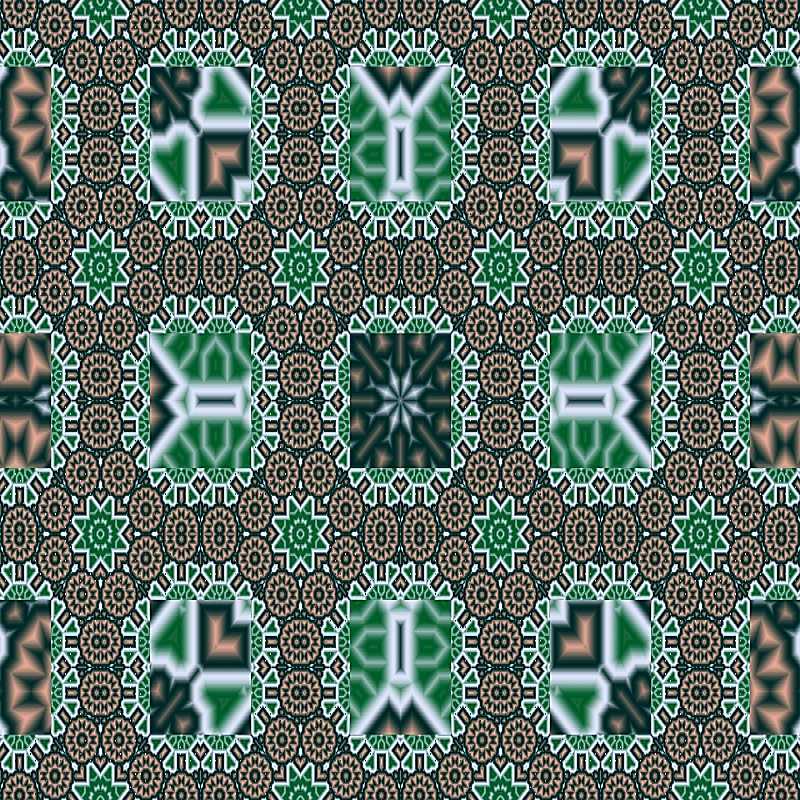
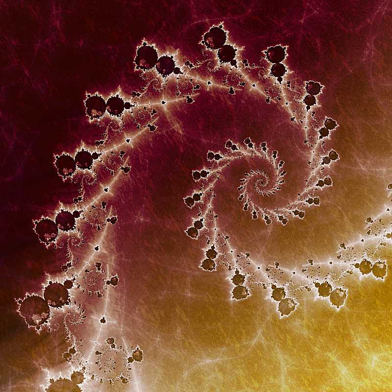
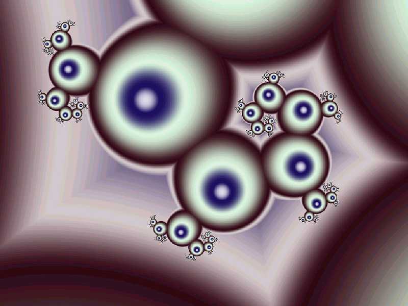
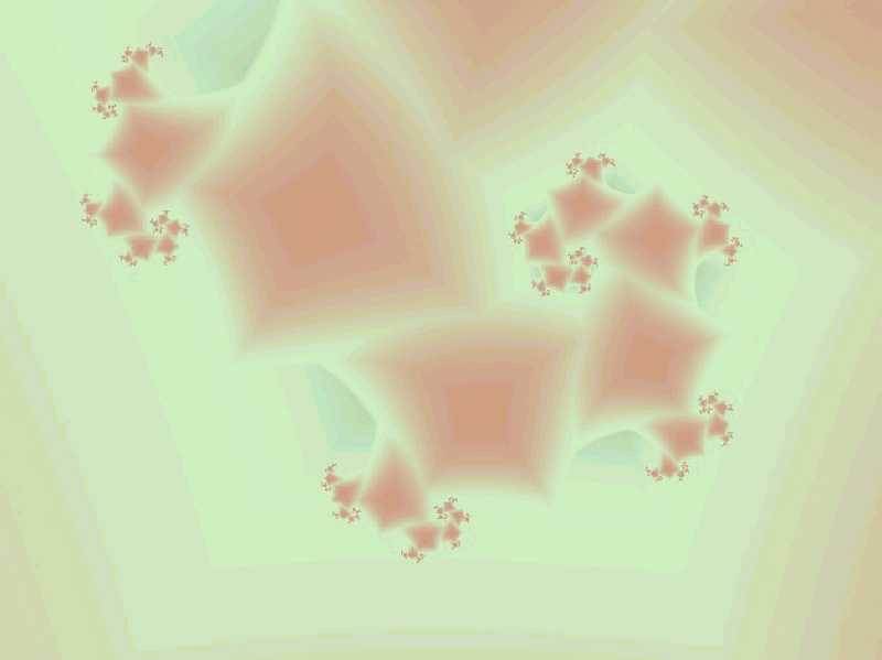
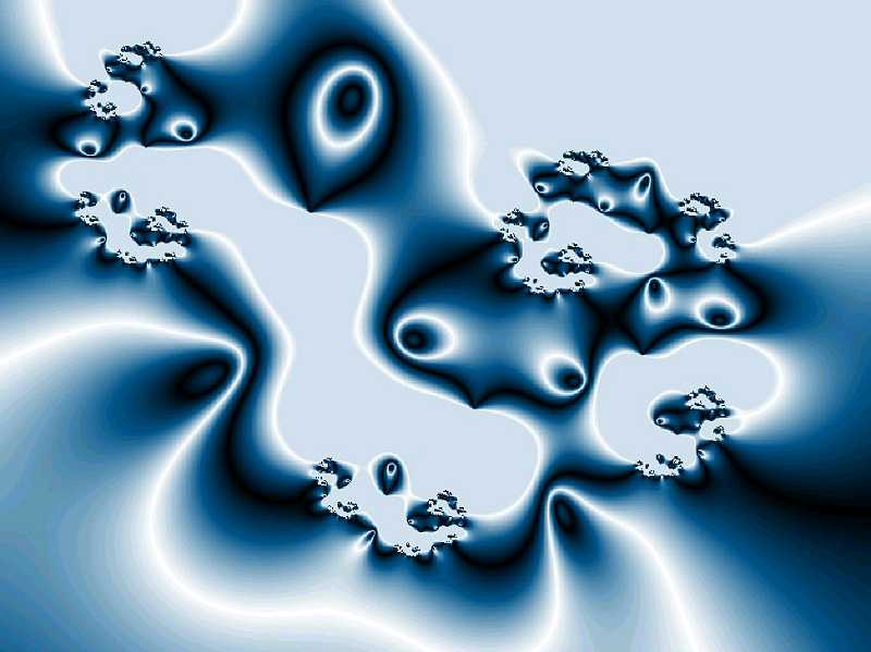
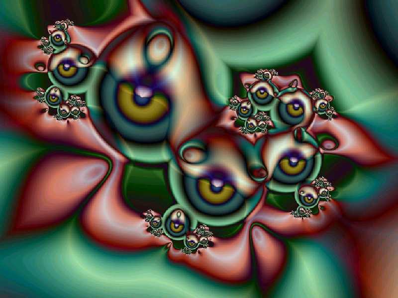
4. Multi layer fractals A more significant technique involves combining techniques. We call these multi layer fractals, and they are the source of some of the richest fractal imagery being produced today. In this way, even a limited collection of fractal coloring algorithms can be combined in almost endless ways, with each combination becoming in effect an entirely new algorithm. Figures 13-15 shows the three layers
of the picture "The eyes of the beholders" using different algorithms,
meanwhile figure 16 shows the final picture with the previous three layers
merged together
References
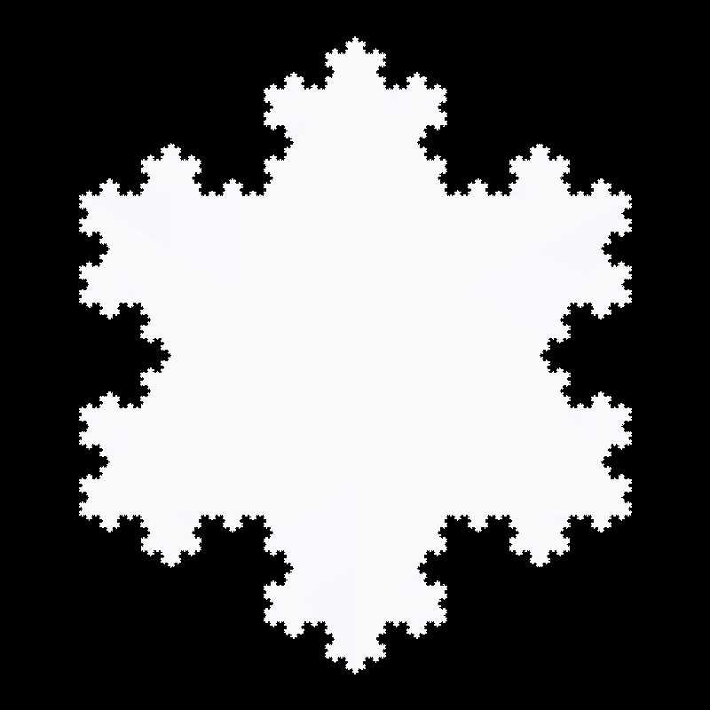 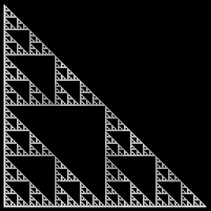
Figures 1-6: Fractal types represented in the
standard way without coloring algorithms. From top left to bottom
Figures 7-12: The same fractal formulas
and parameters of figures 1-6 are repeated here, but
Figures 13-16: "The eyes of the beholders".
The picture is composed by three different images (top) using
|