Estimating mathematical information on Graphs: A Scientific Approach

1  Introduction

Another plan is similar to that taught in elementary school to estimate map distances. One takes a plain piece of paper and mark the distances on that paper and then measures the marked section against a scale given at some other place on the page. This works if the section that needs to be measured on the graph can be compared accurately to a scale somewhere else on the graph. If this section is longer or shorter than the scale one runs into difficulties in determining the differences. Also, one sometimes loses measurement accuracy by transferring measurements so many times. 

A ruler may be a good estimating tool for students working with graphs. The ruler provides a nice straight edge which the students can trace against. It allows measurements that will assist students in measuring more accurately the distance between points on the graph so that they can determine the coordinates of a specific point. One problem with the ruler is that it can be thick and difficult to work with on very small graphs. 

Another option that students may try is a transparent ruler. It is easier to use because students can see through to the paper so they know exactly what they are marking and can see their graph under the ruler while they are drawing their lines. While this is a good instrument for estimating, there is still the problem that the ruler has only one side and in graphing one often needs to measure two coordinates. With a ruler, one has to measure the x-coordinate and then turn the ruler around and measure the y-coordinate. One may also measure inaccurately if the ruler is not positioned properly. These types of rulers can also be quite thick and difficult to work with on small graphs. 

In order to be a little more accurate, students may attempt to use graph paper. While graph paper with large squares is not much better than plain paper, it does provide a good scale if the student is working with a large graph. The incremental markings are quite helpful. However, when working with small graphs it becomes difficult to obtain accurate measurements. One solution is to use graph with the larger squares subdivided by very small incremental markings. These very small markings allow more accurate measurements. Although this is a better plan, there is still the problem that the student is not able to see exactly where the paper is being placed because the paper is opaque. 

What students need in working with these small graphs is a tool that 

• is light and small enough to work with, 
• has sufficiently small incremental markings, 
• has a straight edge for drawing lines, 
• allows the student to see though to the work below, 
• allows easy positioning for accurate measurements, 
• is easy to read, 
• costs less as students will be using it. 

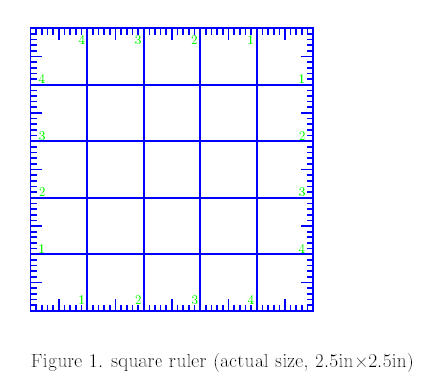
2  Square ruler

One purpose of this method is to foster an awareness of scientific approaches to solving problems. In early education, informal and intuitive measurement is appropriate for inspiring students' natural curiosity. Students usually measure objects with non- standardized units, such as hands or shoes. These informal measuring methods shape young learners' basic mathematical sense and make their mathematical experiences fun. As students continue to explore mathematical concepts and ideas, they gradually discover the necessity of standard units, especially in higher education. A scientific approach to measurement plays a crucial role in problem solving, communicating and reasoning. 

Another purpose of using this square ruler is to help students develop a mathematical way of thinking. This aims at reinforcing the power of mathematics, building desirable attitudes toward learning. It nourishes a logical mode of thought that is fundamental to mathematical discovery and creation. 

Thus the approach to measurement we discuss here not only helps students make reasonably accurate estimations, but also helps them better understand mathematical concepts and ideas. 

We use this tool first to estimate units on the x- and y-axes in terms of units on our square ruler (one unit in our square ruler is .5in). We can estimate the coordinates of a point in terms of units on our square ruler and translate these numbers to actual coordinates on the graph. We can also estimate slopes of (tangent or secant) lines and distances between two points. 

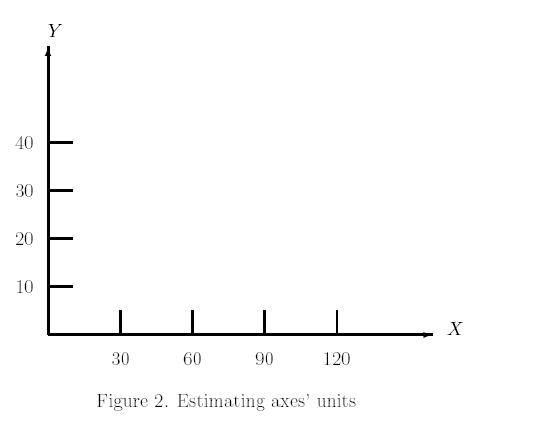
3  Estimating scales on axes

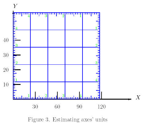
Step 1: 

Place the square ruler on top of the graph. Align its borders with the axes of the graph. Note that the grid on the square ruler makes it easier to recognize any misalignment of the square ruler on the graph and to adjust the square ruler so that the verticle lines are parallel with y-axis and the horizontal lines parallel with x-axis. 

Step 2: 

Read the distance on our square ruler between the marking 0 and 10 of the given graph. In this case, the distance is .85. Thus 10 units on the y-axis are equal to .85 units on our square ruler. Hence, one unit on our square ruler is [10/ .85] = 11.76470588 units on y-axis. 

Read the distance on our square ruler between the number 0 and 30. In this case, the distance is 1.29. Thus 30 units on x-axis are equal to 1.29 units on our square ruler. Hence, one unit on our square ruler is [30/ 1.29] = 23.25581395 units on x-axis. 

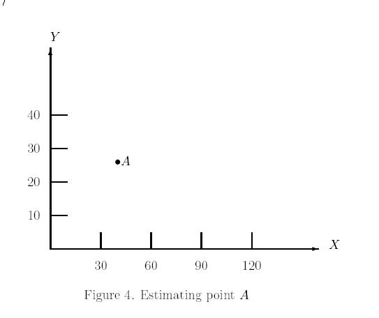
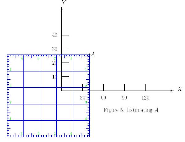
4  Estimating Coordinates

Step 1: 

Estimate the units on axes as described in the previous section: One unit on our square ruler is [10/ .85] = 11.76470588 units on y-axis and [30/ 1.29] = 23.25581395 units on x-axis. 

Step 2: 

Place one corner of the square ruler at the point A, keeping the vertical lines on the square ruler parallel to the y-axis of the graph and the horizontal lines on the square ruler parallel to its x-axis. 

Step 3: 

Read the distance on our square ruler between the y-axis and A. In this case, the distance is 1.7. Thus the x-coordinate of A is [30/ 1.29]1.7 = 39.53488372. 

Step 4: 

Read the distance on our square ruler between the x-axis and A. In this case, the distance is 2.2. Thus y-coordinate of A is [10/ .85]2.2 = 25.88235394. 

Thus A = (39.53,25.88). 
 

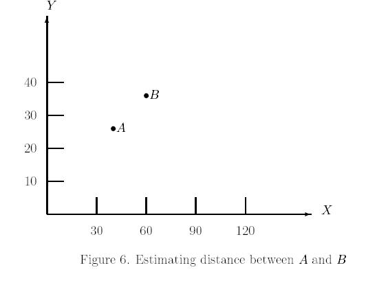
5  Estimating distance

Step 1: 

Estimate the units on axes as described in the previous section: One unit on our square ruler is [10/ .85] = 11.76470588 units on y-axis and [30/ 1.29] = 23.25581395 units on x-axis. 

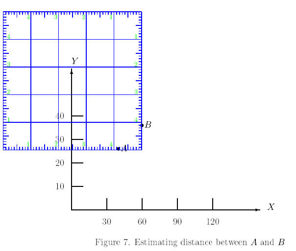
Step 2: 

Place the square ruler in such a way that one point is on the vertical side and the other point is on the horizontal side, keeping the vertical lines on the square ruler parallel to the y-axis of the graph and the horizontal lines on the square ruler parallel to its x-axis. 

Step 3: 

Read the distances on our square ruler between these points and the intersecting corner. (If the square ruler is not wide enough, draw a line between A and B and split the line into parts which can be measured separately and add these measurements.) In this case, the distance for A is .85 and for B is .9. Thus the distance between A and B is Ö{(.85×[10/ .85])²+(.9×[30/ 1.29])²} = 24.86764967. 

Thus the distance between A and B is 24.87. 

6  Estimating Slopes

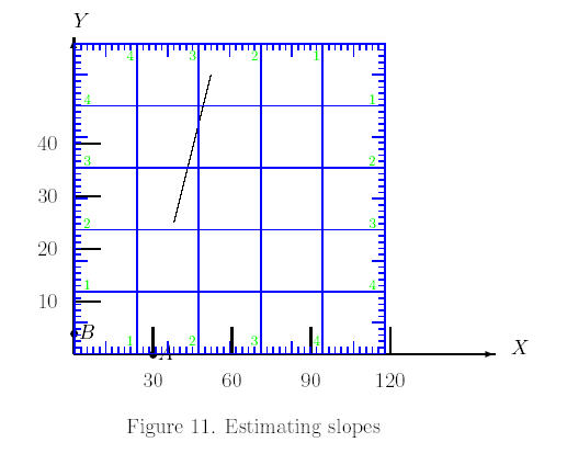
6.1  Slope of a line

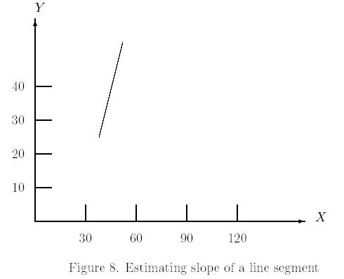
We first estimate the slope on our square ruler. Place the square ruler on the graph, keeping the vertical lines on the square ruler parallel to the y-axis of the graph and the horizontal lines on the square ruler parallel to its x-axis, in such a way that the line meets one horizontal and one vertical side of the square ruler. 

Since line meets the vertical side of the square ruler at 1.2 and the horizontal side of the square ruler at .3, the slope is [1.2/ .3] = 4 with respect to the units on the square ruler. Since we already know, one unit on our square ruler is [10/ .85] units on y-axis and [30/ 1.29] units on x-axis, the slope of the line on the graph is 4×[([10/ .85])/( [30/ 1.29])] = 2.023529412. Thus the slope of the line on the graph is 2.02. 

6.2  Perpendicular lines

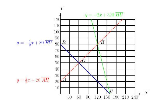
Different scales on axes make it difficult to judge whether two lines are perpendicular by visual inspection. Note that the red ([`AH], y = <sup>1</sup>/<sub>2</sub>x+20) and green ([`HU], y = -2x+320) lines are perpendicular. The red ([`AH], y = <sup>1</sup>/<sub>2</sub>x+20) and blue ([`RU], y = -¹/₂x+80) lines are not perpendicular inspite of their appearance. 

Now, consider the previous problem. Let us try to use perpendicular lines to find the slope of the given line. 

We align our square ruler in such a way that one of the lines overlap on the given line. Note x- and y- intercepts (A and B, respectively) of a perpendicular line. 

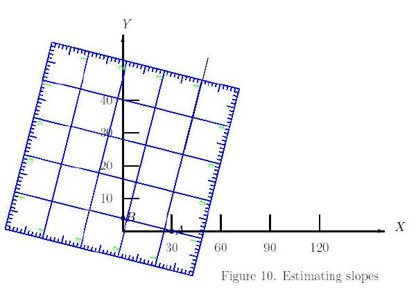
Now find the coordinates of these points as before by aligning the square ruler with the coordinate system. 

Note the A = (30,0) and B = (0,3.8) The line joining A and B is perpendicular to the orignal line in the coordinate system with respect to our square ruler. Hence the original slope is [30/ 3.8]×([([10/ .85])/( [30/ 1.29])])² ~ 2.02. 

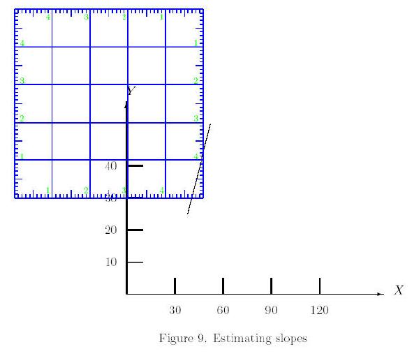
6.3  Slope of the line segment between two points

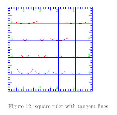
6.4  Tangent lines

The idea is to align one of these arcs with the part of the graph that is around the point where one needs to find a tangent line. Then one can use square ruler lines to figure out the slope. Let us consider the following graph. Let us estimate slope of the tangent line at point marked as ·. 

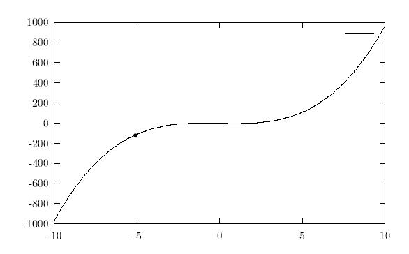
Choose an arc that is closest in shape around the point and place the square ruler in such a way that the arc is aligned on the curve, Note that the intersection point on the curve should match with the point of interest on the graph. 

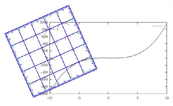
We can use any of the lines parallel to the tangent line to find the slope. In this case, we can use the top line that meets borders of the graph at (-10,800) and (-7.142,1000) (this point was estimated using the method decribed above). Hence the slope of the tangent line is 69.9790063. 

Notice that the accuracy of our measurements is limited by the thickness of the points on the graph. For instance, if a point is a circle with diameter more than .05 inches, then that point certains spans over two consecutive markings on square ruler which clearly compromizes the accuracy. 

7  L^AT_EX code

\documentclass[12pt]{article}

\usepackage{eepic}
\usepackage{color}

\begin{document}

\newcounter{foo}

\newcommand{\gadget}[2]{
\setlength{\unitlength}{.5in}
\begin{picture}(0,0)(#1,#2)
\thinlines
\scriptsize

\color{blue}

% verticle lines

\multiput(0,0)(1,0){6}{\line(0,1){5}}

% horizontal lines

\multiput(0,0)(0,1){6}{\line(1,0){5}}

% bottom

\multiput(0,0)(.1,0){50}{\line(0,1){.1}}
\multiput(0,0)(.5,0){10}{\line(0,1){.2}}


% top

\multiput(0,4.9)(.1,0){50}{\line(0,1){.1}}
\multiput(0,4.8)(.5,0){10}{\line(0,1){.2}}


% left

\multiput(0,0)(0,.1){50}{\line(1,0){.1}}
\multiput(0,0)(0,.5){10}{\line(1,0){.2}}


% right

\multiput(4.9,0)(0,.1){50}{\line(1,0){.1}}
\multiput(4.8,0)(0,.5){10}{\line(1,0){.2}}


% numbers in green

\color{green}

% bottom numbers

\setcounter{foo}{1}
\multiput(.9,0.2)(1,0){4}{\makebox
   (0,0){\arabic{foo}}\addtocounter{foo}{1}}

% top numbers

\setcounter{foo}{4}
\multiput(.9,4.8)(1,0){4}{\makebox
   (0,0){\arabic{foo}}\addtocounter{foo}{-1}}


% left numbers

\setcounter{foo}{1}
\multiput(0.2,1.1)(0,1){4}{\makebox
   (0,0){\arabic{foo}}\addtocounter{foo}{1}}

% right numbers

\setcounter{foo}{4}
\multiput(4.8,1.1)(0,1){4}{\makebox
   (0,0){\arabic{foo}}\addtocounter{foo}{-1}}


%arcs in first line

\color{red}

\put(1,1.51){\arc{1}{.4}{2.7}}
\put(2,1.51){\arc{1}{.6}{2.5}}
\put(3,1.51){\arc{1}{.8}{2.3}}
\put(4,1.51){\arc{1}{1}{2.1}}

% arcs in Second line

\put(1,2.26){\arc{.5}{.4}{2.7}}
\put(2,2.26){\arc{.5}{.6}{2.5}}
\put(3,2.26){\arc{.5}{.8}{2.3}}
\put(4,2.26){\arc{.5}{1}{2.1}}

% arcs in Third line

\put(1,3.11){\arc{.2}{.2}{3.1}}
\put(2,3.11){\arc{0.2}{.4}{2.7}}
\put(3,4.01){\arc{2}{1}{2.1}}

% arcs in Fourth line

\put(1,6.01){\arc{4}{1.2}{1.9}}
\put(4,6.51){\arc{5.0}{1.3}{1.8}}
\color{black}

\end{picture}
}

% change the coordinates according to your convenience

\gadget{2}{2}

\end{document}

8  Acknowledgements

9  References

1. 

Latorre, Kenelly, Fetta, Carpenter, and Harris, Calculus Concepts, An Informal Approach to the Mathematics of Change, brief first edition, Houghton Mifflin, 1998. 

2. 

K. Yashiwara, B. Yashiwara, I. Drooyan, Modeling, Functions, and Graphs, Algebra for College Students, second edition, Brooks/Cole Publishing Company, 1996.